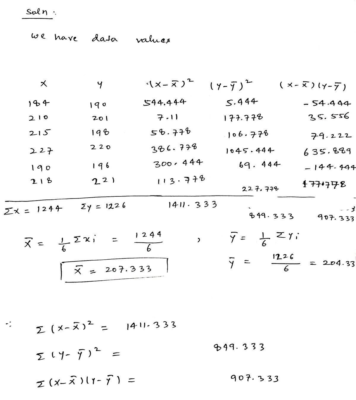
Tire pressure (in kPa) was measured for the left and right front tires on a sample of 6 automobiles.Left (x) Right (y)184190210201215198227220190196218221 e. Compute the covariance and correlation coefficient r between the right tire pressure.f. How do you know the relationship between pressure in the left and right tires is positive.g. What value would a correlation coefficient (r) be close to if there was no (linear) relationship betweenthe 2 tire pressures?

Answered: Image /qna-images/answer/e54af3dc-6807-4b8a-8edd-c652e4b8ef1d.jpg

Answered: e. Compute the covariance and…

MATLAB: An Introduction with Applications

6th Edition

ISBN:9781119256830

Author:Amos Gilat

Publisher:Amos Gilat

Chapter1: Starting With Matlab

Section: Chapter Questions

Problem 1P

See similar textbooks

Similar questions

Dr. Wabld Hamdy given by the following table: y X-4 -2 2 4 --2 0 0.25 0 0 -100 0.25 1 0.25 00 0 2 0.25 0 Find the correlation coefficient between X and Y llu mad and imported automobiles sold
If the linear association between two numerical variables is studied and the correlation coefficient is 0.32, it can be concluded that:a. The relationship between the variables is inverse and weak. b. The percentage of variability observed in the data that is explained by the error is 89.76%. c. The percentage of observed variability in the data that is explained by the model is 32%. d. None is correct Please explain clearly, thank you
A random sample of college students was surveyed about how they spend their time each week. The scatterplot below displays the relationship between the number of hours each student typically works per week at a part- or full-time job and the number of hours of television each student typically watches per week. The correlation between these variables is r = –0.63, and the equation we would use to predict hours spent watching TV based on hours spent working is as follows: Predicted hours spent watching TV = 17.21 – 0.23(hours spent working) Since we are using hours spent working to help us predict hours spent watching TV, we’d call hours spent working a(n) __________________ variable and hours spent watching TV a(n) __________________ variable. The correlation coefficient, along with what we see in the scatterplot, tells us that the relationship between the variables has a direction that is _________________ and a strength that is ______________________. According to the…
Which of the following correlation coefficients indicate the strongest relationship between two variables? A .20 B .87 C .80 D -.95
Find R, R^2 and P Value
Suppose data are collected concerning the weight of a person in pounds and the number of calories burned in 30 minutes of walking on a treadmill at 3.5 miles per hour. How would the value of the correlation coefficient, r, change if all of the weights were converted to kilograms?
As temperature decreases, rates of crime also seem to decrease. Which of the following Pearsons R values represents the strongest possible correlation between these two variables?" -0.5 -1 0.5 1
After gathering data about the number of starfish and measuring the pollution in areas of the ocean you find a negative linear correlation between pollution levels and number of starfish. What can you conclude based on this information? a. There is a confounding variable that is affecting both pollution and starfish. b. As pollution rises the number of starfish falls c. That pollution is causing starfish to die, leading to the negative correlation d. That pollution is supporting starfish, leading to the negative correlation
Please help
Suppose that two variables, x and y, have a correlation coefficient of −0.77. Which of the following statements are true? You must make a selection for each option. Click once to place a check mark for correct answers and click twice to empty the box for the wrong answers. check all that apply There is a strong relationship between these two variables. As x increases, y decreases. The variables have a negative linear relationship. As x increases, y increases. There is a weak relationship between these two variables.
Below is a subset of the data on quality of marriage and quality of parent-child relationship. Using the data provided below, calculate the correlation between the two variables. You should calculate the correlation "by hand" and show your work that led to the solution (take a picture of your hand-written notes and insert it into this document) Quality of marriage Quality of parent-child relationship 1 5 2
A psychologist has calculated the correlation between two variables as 0.9. Which of the following statements is correct? a. The average value of y changes by 0.9 when x is increased by 1. b. The average value of x changes by 0.9 when y is increased by 1. c. The explanatory variable ( x ) explains 0.9 of the variation in the response variable ( y ) d. The explanatory variable ( x ) explains 0.81 of the variation in the response variable ( y )

SEE MORE QUESTIONS

Recommended textbooks for you

MATLAB: An Introduction with Applications

Statistics

ISBN:

9781119256830

Author:

Amos Gilat

Publisher:

John Wiley & Sons Inc

Probability and Statistics for Engineering and th…

Statistics

ISBN:

9781305251809

Author:

Jay L. Devore

Publisher:

Cengage Learning

Statistics for The Behavioral Sciences (MindTap C…

Statistics

ISBN:

9781305504912

Author:

Frederick J Gravetter, Larry B. Wallnau

Publisher:

Cengage Learning

MATLAB: An Introduction with Applications

Statistics

ISBN:

9781119256830

Author:

Amos Gilat

Publisher:

John Wiley & Sons Inc

Probability and Statistics for Engineering and th…

Statistics

ISBN:

9781305251809

Author:

Jay L. Devore

Publisher:

Cengage Learning

Statistics for The Behavioral Sciences (MindTap C…

Statistics

ISBN:

9781305504912

Author:

Frederick J Gravetter, Larry B. Wallnau

Publisher:

Cengage Learning

Elementary Statistics: Picturing the World (7th E…

Statistics

ISBN:

9780134683416

Author:

Ron Larson, Betsy Farber

Publisher:

PEARSON

The Basic Practice of Statistics

Statistics

ISBN:

9781319042578

Author:

David S. Moore, William I. Notz, Michael A. Fligner

Publisher:

W. H. Freeman

Introduction to the Practice of Statistics

Statistics

ISBN:

9781319013387

Author:

David S. Moore, George P. McCabe, Bruce A. Craig

Publisher:

W. H. Freeman

SEE MORE TEXTBOOKS