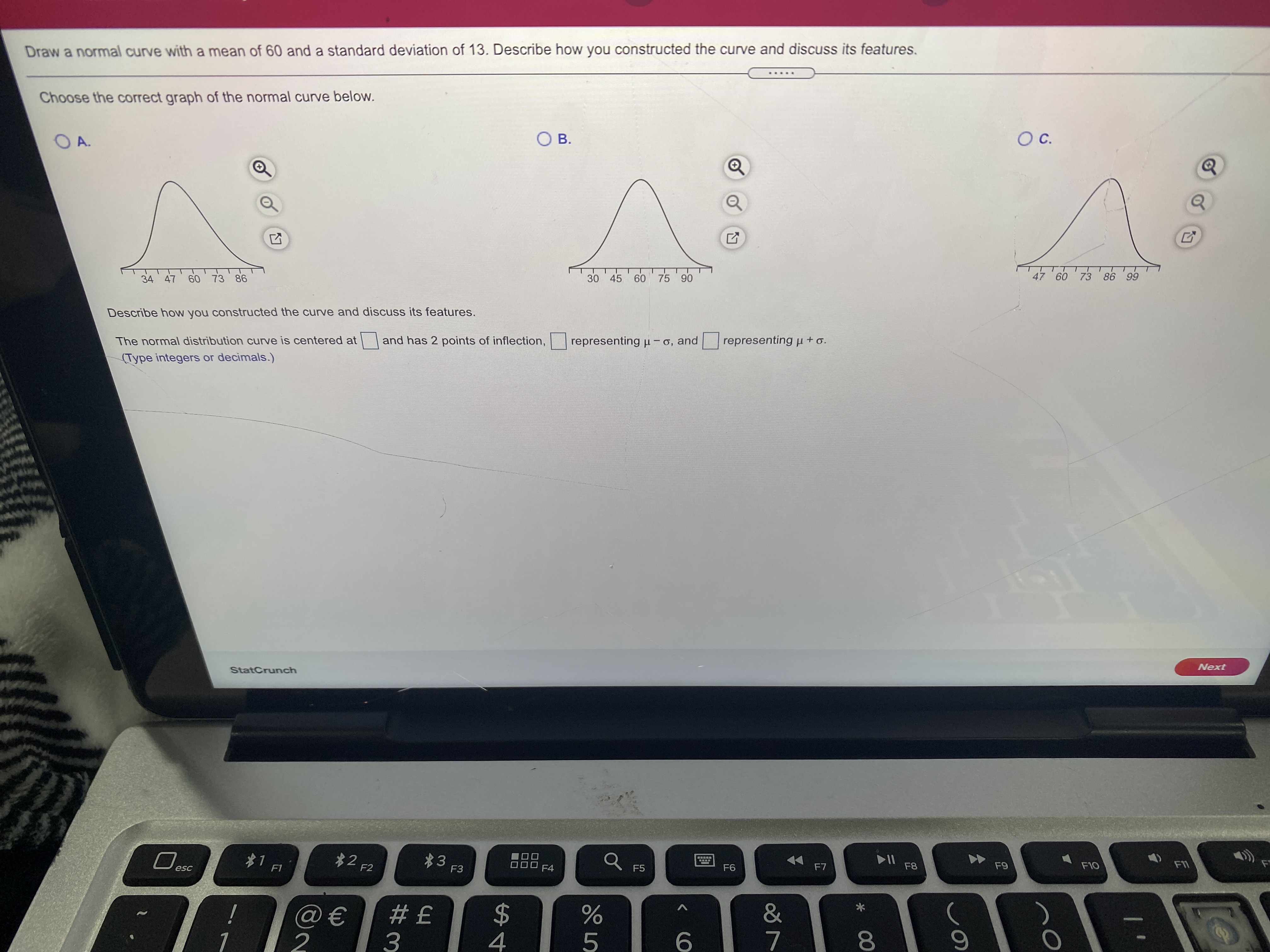
The image contains a question about drawing a normal distribution curve with a mean of 60 and a standard deviation of 13. It asks to choose the correct graph of the normal curve from the given options and to describe how the curve was constructed, including its features.Graph Descriptions:1. Option A: - The graph shows a symmetrical bell curve centered at 50. - The x-axis is labeled with values: 43, 50, and 57.2. Option B: - The graph shows a symmetrical bell curve centered at 65. - The x-axis is labeled with values: 59, 65, and 71.3. Option C: - The graph shows a symmetrical bell curve centered at 73. - The x-axis is labeled with values: 47, 60, and 73.The prompt includes blanks to be filled in with numbers or decimals to specify points of inflection.For educational purposes, the correct graph should be centered at 60, according to the mean provided. The points of inflection for a normal distribution occur at one standard deviation away from the mean (47 and 73 in this case). Therefore, Option C appears to be the most appropriate graph based on the mean and standard deviation given. To construct such a curve:- The mean (µ = 60) is the center of the curve.- Standard deviation (σ = 13) determines the width and spread of the curve, with points of inflection at µ ± σ, which are 47 and 73.

A normal distribution curve is bell shaped curve and it is symmetric about the mean. The normal…

Answered: Draw a normal curve with a mean of 60…

MATLAB: An Introduction with Applications

6th Edition

ISBN:9781119256830

Author:Amos Gilat

Publisher:Amos Gilat

Chapter1: Starting With Matlab

Section: Chapter Questions

Problem 1P

See similar textbooks

Similar questions

the mean is 146, and standard deviation is 35. A score of 181 is how many z-scores above the mean?
Assume that a randomly selected subject is given a bone density test. Those test scores are normally distributed with a mean of 0 and a standard deviation of 1. Find the probability that a given score is less than - 1.34 and draw a sketch of the region. Sketch the region. Choose the correct graph below. OA. OB. OC. OD. -1.34 1.34 -1.34 1.34 -1.34
Assume that a randomly selected subject is given a bone density test. Those test scores are normally distributed with a mean of 0 and a standard deviation of 1. Find the probability that a given score is less than 2.17 and draw a sketch of the region. Sketch the region. Choose the correct graph below. A. -2.17 2.17 The probability is (Round to four decimal places as needed.) B. 2.17 2.17 D. ^ -2.17
One graph in the figure represents a normal distribution with mean u = 7 and standard deviation o = 1. The other graph represents a normal distribution with mean u = 12 and standard deviation o = 1. Determine which graph is which and explain how you know. 12 Choose the correct answer below. O A. Graph A has a mean of u = 12 and graph B has a mean of u =7 because larger mean shifts the graph to the left. O B. Graph A has a mean of u = 12 and graph B has a mean of u =7 because a larger mean shifts the graph to the right. O C. Graph A has a mean of u = 7 and graph B has a mean of u = 12 because a larger mean shifts the graph to the left. O D. Graph A has a mean of u = 7 and graph B has a mean of u = 12 because a larger mean shifts the graph to the right.
T and p value please
Use a table of cumulative areas under the normal curve to find the z-score that corresponds to the given cumulative area. If the area is not in the table, use the entry closest to the area. If the area is halfway between two entries, use the z-score halfway between the corresponding z-scores. If convenient, use technology to find the z-score. 0.051 Click to view page 1 of the table. Click to view page 2 of the table. The cumulative area corresponds to the z-score of (Round to three decimal places as needed.)
Fluorescent lightbulbs have lifetimes that are normally distributed with a mean of 6.2 years and a standard deviation of 1 year. The figure below shows the distribution of lifetimes of fluorescent lightbulbs. Calculate the shaded area under the curve.Express your answer in the decimal form accurately to at least two decimal places. Answer:
Assume that a randomly selected subject is given a bone density test. Those test scores are normally distributed with a mean of 0 and a standard deviation of 1. Draw a graph and find the probability of a bone density test score greater than -1.62. Sketch the region. Choose the correct graph below. O A. 1.62 Q The probability is (Round to four decimal places as needed.) OB. Q -1.62 -1.62 ♫ OD. Q -1.62 1.62 Ε
One graph in the figure represents a normal distribution with mean u= 15 and standard deviation o = 2. The other graph represents a normal distribution with mean u=11 and standard deviation o = 2. Determine which graph is which and explain how you know. A B 11 15 ... Choose the correct answer below. O A. Graph A has a mean of u = 15 and graph B has a mean of u = 11 because a larger mean shifts the graph to the right. O B. Graph A has a mean of u = 11 and graph B has a mean of u= 15 because a larger mean shifts the graph to the left. O C. Graph A has a mean of u = 11 and graph B has a mean of u = 15 because a larger mean shifts the graph to the right. O D. Graph A has a mean of u = 15 and graph B has a mean of u = 11 because a larger mean shifts the graph to the left.
1. Find the area of the shaded region. The graph to the right depicts IQ scores of adults, and those scores are normally distributed with a mean of 100 and a standard deviation of 15. Click to view page 1 of the table. LOADING... Click to view page 2 of the table. LOADING... 75 A graph with a bell-shaped curve, divided into 2 regions by a vertical line. The vertical line extends from the bell curve to the x-axis, and is located on the left half, under the curve. The region on the left of this line is shaded. The x-axis below the vertical line is labeled 75. 2. Find the area of the shaded region. The graph to the right depicts IQ scores of adults, and those scores are normally distributed with a mean of 100 and a standard deviation of 15. 83 A symmetric bell-shaped curve is plotted over a horizontal scale. A vertical line runs from the scale to the curve at labeled…
I can’t figure out formula or answer for bone density
P K @ 2 Listed in the data table are IQ scores for a random sample of subjects with medium lead levels in their blood. Also listed are statistics from a study done of IQ scores for a random sample of subjects with high lead levels. Assume that the two samples are independent simple random samples selected from normally distributed populations. Do not assume that the population standard deviations are equal. Complete parts (a) and (b) below. Click the icon to view the data table of IQ scores. Help me solve this S a. Use a 0.01 significance level to test the claim that the mean IQ scores for subjects with medium lead levels is higher than the mean for subjects with high lead levels. What are the null and alternative hypotheses? Assume that population 1 consists of subjects with medium lead levels and population 2 consists of subjects with high lead levels. F2 W 30² OA H₂: #₁ = 1/₂ H₁: Hy #4₂ OC. Ho: Hy #4₂ H₁: Hy > H₂ The test statistic is (Round to two decimal places as needed.) mmand X…

SEE MORE QUESTIONS

Recommended textbooks for you

MATLAB: An Introduction with Applications

Statistics

ISBN:

9781119256830

Author:

Amos Gilat

Publisher:

John Wiley & Sons Inc

Probability and Statistics for Engineering and th…

Statistics

ISBN:

9781305251809

Author:

Jay L. Devore

Publisher:

Cengage Learning

Statistics for The Behavioral Sciences (MindTap C…

Statistics

ISBN:

9781305504912

Author:

Frederick J Gravetter, Larry B. Wallnau

Publisher:

Cengage Learning

MATLAB: An Introduction with Applications

Statistics

ISBN:

9781119256830

Author:

Amos Gilat

Publisher:

John Wiley & Sons Inc

Probability and Statistics for Engineering and th…

Statistics

ISBN:

9781305251809

Author:

Jay L. Devore

Publisher:

Cengage Learning

Statistics for The Behavioral Sciences (MindTap C…

Statistics

ISBN:

9781305504912

Author:

Frederick J Gravetter, Larry B. Wallnau

Publisher:

Cengage Learning

Elementary Statistics: Picturing the World (7th E…

Statistics

ISBN:

9780134683416

Author:

Ron Larson, Betsy Farber

Publisher:

PEARSON

The Basic Practice of Statistics

Statistics

ISBN:

9781319042578

Author:

David S. Moore, William I. Notz, Michael A. Fligner

Publisher:

W. H. Freeman

Introduction to the Practice of Statistics

Statistics

ISBN:

9781319013387

Author:

David S. Moore, George P. McCabe, Bruce A. Craig

Publisher:

W. H. Freeman

SEE MORE TEXTBOOKS