
MATLAB: An Introduction with Applications
6th Edition
ISBN: 9781119256830
Author: Amos Gilat
Publisher: John Wiley & Sons Inc
expand_more
expand_more
format_list_bulleted
Related questions
Question
Data were collected to explain the number of wins an NFL team has based on the average points per game that they score (PPG)
Based on the regression results, answer the following questions
a) What is the estimated regression equation?
b) What percentage of the wins is explained by PPG?
c) What is the standard error of the error term in the regression equation?
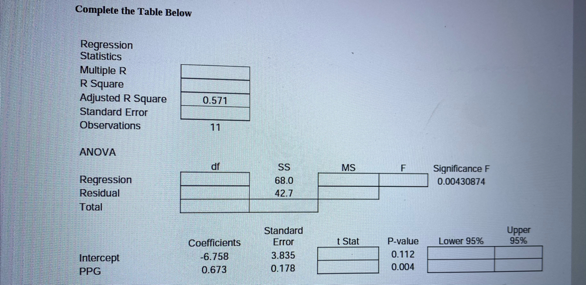

Transcribed Image Text:Complete the Table Below
Regression
Statistics
Multiple R
R Square
Adjusted R Square
0.571
Standard Error
Observations
11
ANOVA
df
SS
MS
F
Significance F
Regression
68.0
0.00430874
Residual
42.7
Total
Upper
95%
Standard
Coefficients
Error
t Stat
P-value
Lower 95%
Intercept
-6.758
3.835
0.112
PPG
0.673
0.178
0.004
Expert Solution
This question has been solved!
Explore an expertly crafted, step-by-step solution for a thorough understanding of key concepts.

This is a popular solution

Trending nowThis is a popular solution!

Step by stepSolved in 4 steps

Knowledge Booster

Similar questions
- The table below gives the number of hours seven randomly selected students spent studying and their corresponding midterm exam grades. Using this data, consider the equation of the regression line, yˆ=b0+b1x, for predicting the midterm exam grade that a student will earn based on the number of hours spent studying. Keep in mind, the correlation coefficient may or may not be statistically significant for the data given. Remember, in practice, it would not be appropriate to use the regression line to make a prediction if the correlation coefficient is not statistically significant. Hours Studying 1 1.5 2 2.5 3 3.5 4.5 Midterm Grades 61 62 75 77 79 83 88 Table Step 1 of 6 : Find the estimated slope, y intercept and correlation cofficient. Round your answer to three decimal places.arrow_forwardA vocational counselor uses the number of days without employment to predict her clients' feelings of self efficacy, measured on a scale of 1 to 5, with higher numbers meaning that clients feel more secure in their job related abilities. The slope of the regression line is –1.02. Which statement is the best interpretation for this finding? a. For every 1-point increase in self-efficacy, there is an associated decrease in the number of days of unemployment. b. For every additional day of unemployment, there is an associated decrease in self-efficacy of 1.02 points. c. The least number of days a person can be unemployed and still feel self-efficacious is 3.98 points d. The decrease in self-efficacy of 1.02 points is caused by each additional day of unemploymentarrow_forwardThe table below gives the number of hours spent unsupervised each day as well as the overall grade averages for five randomly selected middle school students. Using this data, consider the equation of the regression line, yˆ=b0+b1x, for predicting the overall grade average for a middle school student based on the number of hours spent unsupervised each day. Keep in mind, the correlation coefficient may or may not be statistically significant for the data given. Remember, in practice, it would not be appropriate to use the regression line to make a prediction if the correlation coefficient is not statistically significant. Hours Unsupervised 2 3 4 5 6 Overall Grades 94 86 79 71 62 Table Step 1 of 6 : Find the estimated slope, y intercept and correlation coefficient Round your answer to three decimal places. Answerarrow_forward
- Personal wealth tends to increase with age as older individuals have had more opportunitiesto earn and invest than younger individuals. The following data were obtained from a randomsample of eight individuals and records their total wealth (Y) and their current age (X). See attachment for table with figures State the estimated regression line and interpret the slope coefficient.b. What is the estimated total personal wealth when a person is 50 years old?c. What is the value of the coefficient of determination? Interpret it.d. Test whether there is a significant relationship between wealth and age at the 10%significance level. Perform the test using the following six steps.Step 1. Statement of the hypotheses Step 2. Standardised test statistic Step 3. Level of significance Step 4. Decision Rulearrow_forwardThe table below gives the age and bone density for five randomly selected women. Using this data, consider the equation of the regression line, yˆ=b0+b1x, for predicting a woman's bone density based on her age. Keep in mind, the correlation coefficient may or may not be statistically significant for the data given. Remember, in practice, it would not be appropriate to use the regression line to make a prediction if the correlation coefficient is not statistically significant. Age 39 43 46 61 64 Bone Density 352 346 321 314 312 Table Step 1 of 6 : Find the estimated slope. Round your answer to three decimal placesarrow_forwardThe table below gives the age and bone density for five randomly selected women. Using this data, consider the equation of the regression line, yˆ=b0+b1x, for predicting a woman's bone density based on her age. Keep in mind, the correlation coefficient may or may not be statistically significant for the data given. Remember, in practice, it would not be appropriate to use the regression line to make a prediction if the correlation coefficient is not statistically significant. Age 50 59 60 64 68 Bone Density 331 326 325 320 315 Table Step 3 of 6 : Substitute the values you found in steps 1 and 2 into the equation for the regression line to find the estimated linear model. According to this model, if the value of the independent variable is increased by one unit, then find the change in the dependent variable yˆ.arrow_forward
- The table below gives the number of hours spent unsupervised each day as well as the overall grade averages for five randomly selected middle school students. Using this data, consider the equation of the regression line, yˆ=b0+b1x, for predicting the overall grade average for a middle school student based on the number of hours spent unsupervised each day. Keep in mind, the correlation coefficient may or may not be statistically significant for the data given. Remember, in practice, it would not be appropriate to use the regression line to make a prediction if the correlation coefficient is not statistically significant. Hours Unsupervised 0 1 3 4 5 Overall Grades 95 92 85 81 62 Table Step 4 of 6 : Find the estimated value of y when x=3. Round your answer to three decimal places. Answer How to enter your answer (opens in new window)arrow_forwarda) Determine the correlation coefficient, r, and interpret this value in the context of the problem. (Round 4 decimal places)b) Find the equation of the regression line for the given data. (Round the slope and y-intercept 4 decimal places).c) Give a practical interpretation of the slope of the regression line.arrow_forwardThe table below gives the number of hours spent unsupervised each day as well as the overall grade averages for five randomly selected middle school students. Using this data, consider the equation of the regression line, yˆ=b0+b1x, for predicting the overall grade average for a middle school student based on the number of hours spent unsupervised each day. Keep in mind, the correlation coefficient may or may not be statistically significant for the data given. Remember, in practice, it would not be appropriate to use the regression line to make a prediction if the correlation coefficient is not statistically significant. Hours Unsupervised 0 2 3 5 6 Overall Grades 90 89 87 77 61 Table Step 2 of 6 : Find the estimated y-intercept. Round your answer to three decimal places.arrow_forward
arrow_back_ios
arrow_forward_ios
Recommended textbooks for you
- MATLAB: An Introduction with ApplicationsStatisticsISBN:9781119256830Author:Amos GilatPublisher:John Wiley & Sons Inc
 Probability and Statistics for Engineering and th...StatisticsISBN:9781305251809Author:Jay L. DevorePublisher:Cengage Learning
 Statistics for The Behavioral Sciences (MindTap C...StatisticsISBN:9781305504912Author:Frederick J Gravetter, Larry B. WallnauPublisher:Cengage Learning
  Elementary Statistics: Picturing the World (7th E...StatisticsISBN:9780134683416Author:Ron Larson, Betsy FarberPublisher:PEARSON
 The Basic Practice of StatisticsStatisticsISBN:9781319042578Author:David S. Moore, William I. Notz, Michael A. FlignerPublisher:W. H. Freeman
 Introduction to the Practice of StatisticsStatisticsISBN:9781319013387Author:David S. Moore, George P. McCabe, Bruce A. CraigPublisher:W. H. Freeman
MATLAB: An Introduction with Applications
Statistics
ISBN:9781119256830
Author:Amos Gilat
Publisher:John Wiley & Sons Inc
Probability and Statistics for Engineering and th...
Statistics
ISBN:9781305251809
Author:Jay L. Devore
Publisher:Cengage Learning
Statistics for The Behavioral Sciences (MindTap C...
Statistics
ISBN:9781305504912
Author:Frederick J Gravetter, Larry B. Wallnau
Publisher:Cengage Learning
Elementary Statistics: Picturing the World (7th E...
Statistics
ISBN:9780134683416
Author:Ron Larson, Betsy Farber
Publisher:PEARSON
The Basic Practice of Statistics
Statistics
ISBN:9781319042578
Author:David S. Moore, William I. Notz, Michael A. Fligner
Publisher:W. H. Freeman
Introduction to the Practice of Statistics
Statistics
ISBN:9781319013387
Author:David S. Moore, George P. McCabe, Bruce A. Craig
Publisher:W. H. Freeman