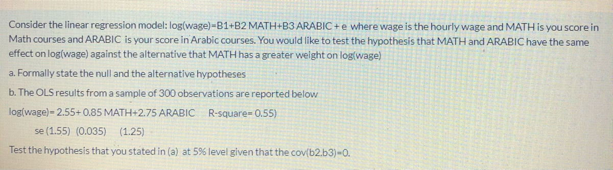
Consider the linear regression model: log(wage)-DB1+B2 MATH+B3 ARABIC +e where wage is the hourly wage and MATH is you score in Math courses and ARABIC is your score in Arabic courses. You would like to test the hypothesis that MATH and ARABIC have the same effect on log(wage) against the alternative that MATH has a greater weight on log(wage) a. Formally state the null and the alternative hypotheses

A well-known university is interested in how salary (in thousands of dollars) is predicted from years of service for faculty and administrative staff.  Below are the estimated regression equations.Faculty (n = 170): ŷ = 60 + 1.1xAdmin. (n = 155): ŷ = 57 + 1.5x a) How much would a faculty member be earning after 5 years of service? b) In how many years will an administrator earn the same amount as in a)?

A company studying the productivity of its employees on a new information system was interested in determingg if the age (X) of data entry opeertors influenced the number of completed entries made per hour (Y). The regression equation is y = 14.374 - 0.145x Suppose the acyual completed entries per hour for an operator who is 35 years old was 8. The residual is:

An advertising firm wishes to demonstrate to potential clients the effectiveness of the advertising campaigns it has conducted. The firm is presenting data from 12 recent campaigns, with the data indicating an increase in sales for an increase in the amount of money spent on advertising. In particular, the least-squares regression equation relating the two variables cost of advertising campaign (denoted by x and written in millions of dollars) and resulting percentage increase in sales (denoted by y) for the 12 campaigns is y = 6.18 +0.14x, and the standard error of the slope of this least-squares regression line is approximately 0.10. Using this information, test for a significant linear relationship between these two variables by doing a hypothesis test regarding the population slope B₁. (Assume that the variable y follows a normal distribution for each value of x and that the other regression assumptions are satisfied.) Use the 0.10 level of significance, and perform a two-tailed…

A sports statistician was interested in the relationship between game attendance (in thousands) and the number of wins for baseball teams. Information was collected on several teams and was used to obtain the regression equation ŷ = 4.9x + 15.2, where x represents the attendance (in thousands) and ŷ is the predicted number of wins. What is the predicted number of wins for a team that has an attendance of 17,000? 83.3 wins 98.5 wins 258.4 wins 263.3 wins

Consider the following hypothetical regression:   FRIES = 22.5 + 0.08*TRAFFIC + 9.1*COUPON? + -1.1*TEMP where FRIES is the number of pounds of fries a restaurant sells in a week, TRAFFIC is the number of people who walked by the restaurant that week (foot traffic), COUPON? is a dummy variable of if the restaurant offered a coupon or not that week (1=coupon, 0=no coupon); and TEMP is the average high that week, measured in Fahrenheit. All variables are statistically significant. If the average high is expected to be 4 degrees warmer next week, how should FRIES change? 1   Increase by 18.1 pounds 2   Decrease by 4.4 pounds 3   It is impossible to tell without knowing the values of TRAFFIC and COUPON?. 4   Increase by 4.4 pounds 5   Increase by 26.9 pounds

A group of scientists wants to determine the efficacy of a vaccine. To do they recruited 1000 subjects. Two months ago 300 random subjects received the vaccine T = 1. The other 700 received a placebo T = 0. The scientist also measured if the subjects became infected with the virus Y = 1 or not Y = 0 in the last 2 months. They plan to test the efficacy of the vaccine by running the following regression: Y = Bo + Bit tu Which of the following statements is FALSE: Select one: a. This model will generate biased estimates because it does not control for many omitted variables Ob. The fact that more people receive the placebo than the vaccine will not generate bias Scientists do not need to observe the initial health status of the subjects to get unbiased estimates because the assignment of the vaccine was random O d. A negative B₁ would indicate that the vaccine is effective c.

Assume there is a positive linear correlation between the variable R (Return rate in percent of a financial investment) and the variable t (age in years of the investment) given by the regression equation R= 2.3t + 4.8  A. Without further information, can we assume there is a cause-and-effect relationship between the return rate and the age of the investment? B. If the investment continues to grow at a constant rate, what is the expeted return rate when the investment is 7 years old? C. If the investment continues to grow at a constant rate, how old is the investment when the return rate is 30%?