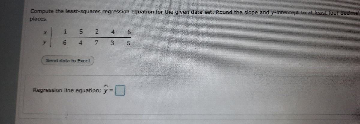
Compute the least-squares regression equation for the given data set. Round the slope and yFintercept to at least four decimal places. 4 y 4. 7. 3 Send data to Excel Regression line equation: y =

Refer to the Baseball 2018 data, which reports information on the 2018 Major League Baseball season. Let attendance be the dependent variable and total team salary be the independent variable. Determine the regression equation and answer the following questions. Click here for the Excel Data Filea-1. Draw a scatter diagram.1. On the graph below, use the point tool to plot the point corresponding to the Attendance and its team salary (Salary 1).2. Repeat the process for the remainder of the sample Salary 2, Salary 3, … ).3. To enter exact coordinates, double-click on the point and enter the exact coordinates of x and y.   a-2. From the diagram, does there seem to be a direct relationship between the two variables?multiple choice 1 Yes No b. What is the expected attendance for a team with a salary of $100.0 million? (Round your answer to 4 decimal places.)   c. If the owners pay an additional $30 million, how many more people could they expect to attend? (Round your answer to 3…

Report the equation of the regression line and interpret it in the context of the problem

Part a: Make a scatter plot and determine which type of model best fits the data.Part b: Find the regression equation.Part c: Use the equation from Part b to determine y when x = 1.5.

Write out the full linear model including all dummy variables below. Don’t worry about estimating regression coefficients just yet. Feel free to abbreviate variable names so long as they are clearly distinguishable.

Fill in the blanks. a. Multicollinearity is considered to be severe if the VIF for one or more predictor variables is ______. or greater. b. If the coefficient of multiple determination for the regression of the predictor variable x11 on all the other predictor variables in a regression equation is 0.6, then the VIF for x1 is ______. c. The effect of multicollinearity in a polynomial regression analysis can be reduced by ______. the predictor variable.

The data show the bug chirps per minute at different temperatures. Find the regression​ equation, letting the first variable be the independent​ (x) variable. Find the best predicted temperature for a time when a bug is chirping at the rate of 3000 chirps per minute. Use a significance level of 0.05. What is wrong with this predicted​ value?   Chirps in 1 min 924 1150 840 1166 1087 930   Temperature ​(°​F) 77.5 84.6 74.1 91 79.6 79.7 What is the regression​ equation? What is the best predicted temperature for a time when a bug is chirping at the rate of 3000 chirps per​ minute? What is wrong with this predicted​ value? Choose the correct answer below. A. It is unrealistically high. The value 3000 is far outside of the range of observed values. B. The first variable should have been the dependent variable. C. It is only an approximation. An unrounded value would be considered accurate. D. Nothing is wrong with this value. It can be…

The data show the chest size and weight of several bears. Find the regression​ equation, letting chest size be the independent​ (x) variable. Then find the best predicted weight of a bear with a chest size of 58 inches. Is the result close to the actual weight of 662 pounds? Use a significance level of 0.05. Chest size (Inches) 46 57 53 41 40 40 Weight (Pounds) 384 580 542 358 306 320

Compute the least-squares regression equation for the given data set. Round the slope and yFintercept to at least four decimal places. 4 y 7. 3. Send data to Excel Regression line equation: y =|