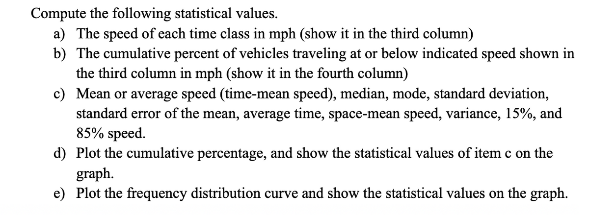
Compute the following statistical values. a) The speed of each time class in mph (show it in the third column) b) The cumulative percent of vehicles traveling at or below indicated speed shown in the third column in mph (show it in the fourth column) c) Mean or average speed (time-mean speed), median, mode, standard deviation, standard error of the mean, average time, space-mean speed, variance, 15%, and 85% speed. d) Plot the cumulative percentage, and show the statistical values of item c on the graph. e) Plot the frequency distribution curve and show the statistical values on the graph.

Represent the Data Set X= {6,5,9,7,7,8, 5, 10,8, 6, 8, 8, 4, 7,8, 7,6} with a bar chart and determine; a) Its mode and its range. b) Its median, upper & lower quartiles and inter-quartile range. c) Its mean, variance and standard deviation.

Solve for C)

Find the mean absolute deviation of the data below 10,15,9,8,7,11,14,8,10,12

The table below gives the weight measurements of 200 castings: Weight in Kg. No. of Castings Weight in Kg. No. of Castings 81-90 2 141-150 37 91-100 5 151-160 29 101-110 13 161-170 11 111-120 20 171-180 3 121-130 30 181-190 131-140 49 Calculate arithmetic mean, median, mode and standard deviation.

calculate the standard deviation of the data shown, 27.7, 10.8, 10.6, 21.1,22.1. round to 2 decimal places

If data set A has a larger standard deviation than data set B, data set A is more spread out than data set B. A. True B. False

the driving distances (miles) to wor of 30 people are shown below. assume the population standard deviation is 8 miles. Find: 12, 9, 7, 3, 27, 21, 2, 30, 7, 4, 1, 10, 2, 9, 2, 28, 7, 10, 13, 6, 13, 7, 3, 13, 6, 6, 3, 13 ,12, 16, 18 a) the point estimate of the population mean  b) the margin of error for a 95% confidence interval  c) contruct a 95% confidence interval for the population mean.

Identify the statistic that is used to estimate a. a population mean.b. a population standard deviation.

the "age" variable measures participants age in years. use spss to calculate the mean age of the sample. the mean age of students in this data set is ____years.  enter your answer rounded to two decimal places.