
MATLAB: An Introduction with Applications
6th Edition
ISBN: 9781119256830
Author: Amos Gilat
Publisher: John Wiley & Sons Inc
expand_more
expand_more
format_list_bulleted
Related questions
Question
Calculate the lower bound of table 1.1 since the values are unreasonable. Refer to table 1.9 for the trial results for recalculation

Transcribed Image Text:Raw Data, Table 1.0
Diameter of
the hole
(mm)
.
6
7
8
9
10
8
9
10
Time taken to drain (s)
((3s.f)
=
Trial
1
71.4
53.3
63
54.2 49.5 54.9 54.7
42.2 42.3 39.6 42.7 41.7
36.5 38.1 37.7
38.2
37.6
Average =
Trial
2
Trial
3
70.2 83.4
Trial
4
81.6
61.8 63.5 62.4
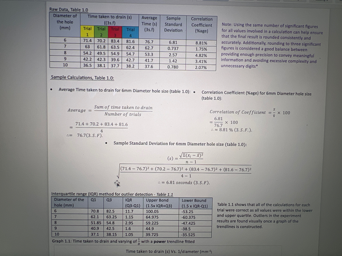
Sample Calculations, Table 1.0:
Average Time taken to drain for 6mm Diameter hole size (table 1.0):.
71.4 + 70.2 + 83.4 +81.6
4
Sum of time taken to drain
Number of trials
= 76.7(3.S.F).
●
Average Sample
Time (s) Standard
(3s.f) Deviation
76.7
62.7
(Q3-Q1)
11.7
51.85 54.8
1.15
2.95
1.6
37.1 38.15 1.05
40.9 42.5
70.8 82.5
62.1 63.25
6,81
0.737
2.57
1.42
0.780
Graph 1.1: Time taken to drain and varying of
D
Correlation
Coefficient
(%age)
8.81%
1.75%
4.82%
3.41%
2.07%
(s) =
Interquartile range (IQR) method for outlier detection - Table 1.1
Diameter of the
Q3
Upper Bond
hole (mm)
Q1
IQR
(1.5x IQR+Q3)
Lower Bound
(1.5 x IQR-Q1)
-53.25
6
100.05
7
64.975
-60.375
-47.425
59.225
44.9
-38.5
39.725
-35.525
with a power trendline fitted
Correlation Coefficient (%age) for 6mm Diameter hole size
(table 1.0):
Sample Standard Deviation for 6mm Diameter hole size (table 1.0):
√Σ(x₁ - x)²
n-1
Note: Using the same number of significant figures
for all values involved in a calculation can help ensure
that the final result is rounded consistently and
accurately. Additionally, rounding to three significant
figures is considered a good balance between
providing enough precision to convey meaningful
information and avoiding excessive complexity and
unnecessary digits*
Correlation of Coefficient
6.81
76.7
=
(71.4-76.7)² + (70.2 - 76.7)² + (83.4 -76.7)² + (81.6- 76.7)²
4-1
= 6.81 seconds (3.S.F).
x 100
8.81 % (3.S.F.).
Time taken to drain (s) Vs. 1/diameter (mm-¹)
=
S
x 100
Table 1.1 shows that all of the calculations for each
trial were correct as all values were within the lower
and upper quartile. Outliers in the experiment
results are found visually once a graph of the
trendlines is constructed.
Expert Solution
This question has been solved!
Explore an expertly crafted, step-by-step solution for a thorough understanding of key concepts.

Step by stepSolved in 3 steps

Knowledge Booster

Similar questions
- The board of examiners that administers the real estate brokerʹsexamination in a certain state found that the mean score on the test was 487 and the standard deviation was 72. If the board wants to set the passing score so that only the best 80% of all applicants pass, what is the passing score? Assume that the scores are normally distributedarrow_forwardmatch the following(1-a, 2-c, etc.)arrow_forwardIt is known that the mean time taken for a taco delivery from a taco shop is 18.4 minutes and the standard deviation is 2.4 minutes. The taco shop wants to promote the business by guaranteeing a maximum waiting time for its cus- tomers. If a taco delivery is not serviced within that period, the customer will receive 42% discount on the charges. The company wants to limit this dis- count to at most 5% of the customers. What should the maximum guaranteed waiting time be?arrow_forward
- Suppose that you have created a contingency table comparing the restaurants that students ate at and whether they got food poisoning. You calculate a chi-square value and use it to determine a level a significance for this contingency table. State the null hypothesis that this test would be examining.arrow_forwardDiscuss the assumptions for one-sampled t-test and why they are important.arrow_forwardYou are testing that the mean speed of your cable Internet connection is 100 Megabits per second. State the null and alternative hypotheses.arrow_forward
- Assume the below life table was constructed from following individuals who were diagnosed with a slow-progressing form of prostate cancer and decided not to receive treatment of any form. Calculate the survival probability at year 1 using the Kaplan-Meir approach and interpret the results. Time in Years Number at Risk, Nt Number of Deaths, Dt Number Censored, Ct Survival Probability 0 20 1 1 20 3 2 17 1 3 16 2 1 The probability of surviving 1 year after being diagnosed with a slow-progressing form of prostate cancer is .85. The probability of surviving 1 year after being diagnosed with a slow-progressing form of prostate cancer is .85 for the individuals being followed in this study. The probability of surviving 1 year after being diagnosed with a slow-progressing form of prostate cancer is .85 for individuals who decided against all forms of treatment. The probability of surviving 1 year after being…arrow_forwardA man who moves to a new city sees that there are two routes he could take to work. A neighbor who has lived there a long time tells him Route A will average 5 minutes faster than Route B. The man decides to experiment. Each day he flips a coin to determine which way to go, driving each route 20 days. He finds that Route A takes an average of 45 minutes, with standard deviation 3 minutes, and Route B takes an average of 49 minutes, with standard deviation 5 minutes. Histograms of travel times for the routes are roughly symmetric and show no outliers. Complete parts a and b. (...) a) Find a 95% confidence interval for the difference between the Route B and Route A commuting times, (µÂ ¯ µÃ) - The confidence interval is (.). (Round to two decimal places as needed.)arrow_forwardSuppose that you want to compare the means of several treatments in a randomized block ANOVA. If given the choice between using the randomized block ANOVA test and the Friedman test, which one would you choose if outliers occur in the sample data? Explain your answer.arrow_forward
- Assume the below life table was constructed from following individuals who were diagnosed with a slow-progressing form of prostate cancer and decided not to receive treatment of any form. Calculate the survival probability at year 1 using the Kaplan-Meir approach and interpret the results. Time in Years Number at Risk, Nt Number of Deaths, Dt Number Censored, Ct Survival Probability 0 20 1 1 20 3 2 17 1 3 16 2 1 A) The probability of surviving 1 year after being diagnosed with a slow-progressing form of prostate cancer is .85. B) The probability of surviving 1 year after being diagnosed with a slow-progressing form of prostate cancer is .85 for the individuals being followed in this study. C) The probability of surviving 1 year after being diagnosed with a slow-progressing form of prostate cancer is .85 for individuals who decided against all forms of treatment. D) The probability of surviving 1 year…arrow_forwardThe researcher would like to determine if these data provide convincing evidence that the true mean amount of time volunteers who were given training held their breath is greater than volunteers without training. Let μ1 = the true mean amount of time that volunteers who were given training held their breath and μ2 = the true mean amount of time that volunteers without training held their breath. What are the appropriate hypotheses?arrow_forwardThe time needed to find a parking space is normally distributed with a mean of 20 minutes and a standard deviation of 5.18 minutes. 90% of the time, it takes less than how many minutes to find a parking space?arrow_forward
arrow_back_ios
arrow_forward_ios
Recommended textbooks for you
- MATLAB: An Introduction with ApplicationsStatisticsISBN:9781119256830Author:Amos GilatPublisher:John Wiley & Sons Inc
 Probability and Statistics for Engineering and th...StatisticsISBN:9781305251809Author:Jay L. DevorePublisher:Cengage Learning
 Statistics for The Behavioral Sciences (MindTap C...StatisticsISBN:9781305504912Author:Frederick J Gravetter, Larry B. WallnauPublisher:Cengage Learning
  Elementary Statistics: Picturing the World (7th E...StatisticsISBN:9780134683416Author:Ron Larson, Betsy FarberPublisher:PEARSON
 The Basic Practice of StatisticsStatisticsISBN:9781319042578Author:David S. Moore, William I. Notz, Michael A. FlignerPublisher:W. H. Freeman
 Introduction to the Practice of StatisticsStatisticsISBN:9781319013387Author:David S. Moore, George P. McCabe, Bruce A. CraigPublisher:W. H. Freeman
MATLAB: An Introduction with Applications
Statistics
ISBN:9781119256830
Author:Amos Gilat
Publisher:John Wiley & Sons Inc
Probability and Statistics for Engineering and th...
Statistics
ISBN:9781305251809
Author:Jay L. Devore
Publisher:Cengage Learning
Statistics for The Behavioral Sciences (MindTap C...
Statistics
ISBN:9781305504912
Author:Frederick J Gravetter, Larry B. Wallnau
Publisher:Cengage Learning
Elementary Statistics: Picturing the World (7th E...
Statistics
ISBN:9780134683416
Author:Ron Larson, Betsy Farber
Publisher:PEARSON
The Basic Practice of Statistics
Statistics
ISBN:9781319042578
Author:David S. Moore, William I. Notz, Michael A. Fligner
Publisher:W. H. Freeman
Introduction to the Practice of Statistics
Statistics
ISBN:9781319013387
Author:David S. Moore, George P. McCabe, Bruce A. Craig
Publisher:W. H. Freeman