Part A
The next questions are in relation to recent study of house prices in Sydney. The variables investigated are:
1 SalePrice Selling Price in Thousands of dollars
2 Distance Distance from Sydney CBD in Kilometers
3 LandSize Land size in square meters
4 Building Area Building Area Construction in square meters
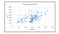
Research Question: Is there a relation between Price of the house and land size?
The output below presents the relation between Price of the house (in thousands of dollars) and land size.The
>results1 <- lm(SalePrice ~ LandSize)
>results1
Call: lm(formula = SalePrice ~ LandSize)
Coefficients:
(Intercept) LandSize
493.4233 1.5821
>summary(results1)
Call: lm(formula = SalePrice ~ LandSize)
Coefficients:
Estimate Std. Error t value Pr(>|t|)
(Intercept) 493.42 119.47 4.13 0.0001
LandSize 1.5821 0.1926 **** *****
Residual standard error: 483.86 on 182 degrees of freedom
Multiple R-squared: 0.52, Adjusted R-squared: 0.2665
- Comment on the relation between the two test marks using the scatterplot.(Choose one from below)
-If the linear equation between the Sale Price and Land Sale is given as:
What is the value of a from the output above (2 dp)
=
What is the value of b from the output above (2 dp)
=
Is there a relation between Sale Price and Land Size?
Perform an appropriate hypothesis test to answer the above research question:
- The null and alternative hypotheses are (Choose one from below)
.
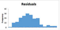
- How can you justify the assumption for this test? (Choose one from below)
-Calculate and give the value of the t test statistic? (3 dp): (Choose one from below)
| 205.9 | 0.193 | 8.215 | 4.130 | 4.224 |
- What are the degrees of freedom? (Choose one from below)
| 46 | 184 | 50 | 26 | 182 |


1) From the scatter plot, there appears to be a moderate positive linear relation between the two variables.
2) a=493.42 and b=1.58
3) H0: β = 0, H1: β ≠ 0
4) The shape of the histogram indicates that the scores may be from a normal distribution and/or the sample size is reasonably large so the sample mean will be from a normal population.
Step by stepSolved in 2 steps

- If the level of employee satisfaction drops below 0.60 overall, then there is a belief that there may be a serious problem with morale in that department. There have been rumors that the Human Resources department (hr in the data file) may be having just such issues. Using a statistical package, test to determine if the mean employee satisfaction level in the Human Resources department is less than 0.60. 1. Is satisfaction level a qualitative or quantitative variable? 2. Graph the employee satisfaction level for the Human Resources department with an appropriate graph and calculate statistics appropriate for this type of data. 3. Conduct the appropriate hypothesis test using the following steps. a. Determine the null and alternative hypotheses. b. Use a significance level of a = 0.05. c. Validate the assumptions of the hypothesis test, identify the appropriate test statistic, and compute its value. d. Determine the P-value. e. Make a decision to reject or fail to reject the null…arrow_forwardin this question I am asking, only answer exercise 6-76 preferably.arrow_forwardYou want to know if relationship between Private Attorney and Amount is consistent for females and males Amount vs. Gender Hint: Graph > Graph Bullder; Drag and drop Amount in Y, Gender in X, and Private Attorney in Group X. Click on the box plot icon at the top. Or, right-click in the graph and select Points > Change Private Attormey Not Private Private Overlay 000000 Color to > Box Plot. What is your conclusion? Interval 700000 O Amount O l a private atorney was used the payout was generaly higher for both male and female patients O Ita private attorney was used the payout was generally lower for male and higher for temale patients 500000 ADOD00 O fa private atnorney was used the payout wan generaly lower for both male and temale patients 300000 OHa pivate attorney was used the payout was generaly higher for male and kower for fermale patients 200000 100000 Femee Mae Femaie Mae Gender Question 9arrow_forward
- 1, If there is a non-linear relationship between a predictor variable and an outcome, what kind of shape would the scatterplot resemble? explain detail. along with the scatter plot. 2.. Why would the scatterplot resemble a funnel/triangle if the assumption of homoscedasticity is violated? explain with figures.arrow_forwardThe amount of time adults spend watching television is closely monitored by firms because this helps to determine advertising pricing for commercials. Complete parts (a) through (d). C (a) Do you think the variable "weekly time spent watching television" would be normally distributed? If not, what shape would you expect the variable to have? A. The variable "weekly time spent watching television" is likely skewed right, not normally distributed. OB. The variable "weekly time spent watching television" is likely symmetric, but not normally distributed. O C. The variable "weekly time spent watching television" is likely skewed left, not normally distributed. O D. The variable "weekly time spent watching television" is likely normally distributed. O E. The variable "weekly time spent watching television" likely uniform, not normally distributed. (b) According to a certain survey, adults spend 2.45 hours per day watching television on a weekday. Assume that the standard deviation for "time…arrow_forwardPlz asaparrow_forward
- Resources Faculty Course Moodle Help Library English (U (en_us) Request Request Services stion The maximum annual windspeeds (in meters per yet vered second) in Hong Kong over a 45-year period is displayed in a histogram below. (Source: Renewable Energy Journal, 2007) ts out of lag Histogram of windspeed tion 14 12 30 40 50 60 windspeed Which of the following statistics is most appropriate for measuring the variation (spread) in the distribution shown of maximum annual windspeeds in Hong Kong? Select one: a. IQR b. Median C. Standard deviation d. Range frequencyarrow_forwardences in your response. Investigation 2: Songs from Spotify - Mode and Popularity A random sample of 3439 songs was selected from the Spotify database and twelve variables were measured for each song. Remember, the Mode variable indicates the type of scale the song's melodic content is derived from (Major or Minor). Popularity is on a scale of 0 to 100 and songs with higher numbers are more popular. Let us now investigate whether Major songs are significantly more "Popular" than Minor songs. Let us define "Popular" as songs that earned a popularity rating of 50 or higher. From the random sample of songs, there were 1964 Major songs and of those 853 were rated "Popular." In addition, there were 1475 Minor songs and of those 587 were rated "Popular." In this invesligation we will subtract (Major - Minor). a) Define the population parameter using context and symbols in one complete sentence. b) State the hypotheses using the claim. c) Check the specific conditions necessary to consider…arrow_forwardIf the data points do not lie in a straight line, there is no relationship between the variables True Falsearrow_forward
- 8 Here we are talking about quality control and the control charts depends variable or attribute . THE TITLE IS ... GYMS .... WE NEED THIS CHARACTERSTICS ( 3 THINGS ENOUGH ) NOTE ; TALKING ABOUT .... GYMS .... Define the quality characteristics and identify whether they are variable or attribute. Explain in detail how they are related to the quality of the product/servicearrow_forwardea surface temperature26.726.726.626.626.626.626.526.526.326.326.126.1Growth0.850.850.850.850.790.790.860.860.890.890.920.92 Make a scatterplot. Which is the explanatory variable? The plot shows a negative linear pattern. Explanatory Variable:arrow_forwardPART D TO BE ANSWERED! Thank you!arrow_forward
 MATLAB: An Introduction with ApplicationsStatisticsISBN:9781119256830Author:Amos GilatPublisher:John Wiley & Sons Inc
 Probability and Statistics for Engineering and th...StatisticsISBN:9781305251809Author:Jay L. DevorePublisher:Cengage Learning
 Statistics for The Behavioral Sciences (MindTap C...StatisticsISBN:9781305504912Author:Frederick J Gravetter, Larry B. WallnauPublisher:Cengage Learning
 Elementary Statistics: Picturing the World (7th E...StatisticsISBN:9780134683416Author:Ron Larson, Betsy FarberPublisher:PEARSON
 The Basic Practice of StatisticsStatisticsISBN:9781319042578Author:David S. Moore, William I. Notz, Michael A. FlignerPublisher:W. H. Freeman
 Introduction to the Practice of StatisticsStatisticsISBN:9781319013387Author:David S. Moore, George P. McCabe, Bruce A. CraigPublisher:W. H. Freeman


