A First Course in Probability (10th Edition)
10th Edition
ISBN: 9780134753119
Author: Sheldon Ross
Publisher: PEARSON
expand_more
expand_more
format_list_bulleted
Question
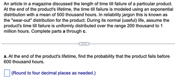
Transcribed Image Text:An article in a magazine discussed the length of time till failure of a particular product.
At the end of the product's lifetime, the time till failure is modeled using an exponential
distribution with a mean of 500 thousand hours. In reliability jargon this is known as
the "wear-out" distribution for the product. During its normal (useful) life, assume the
product's time till failure is uniformly distributed over the range 200 thousand to 1
million hours. Complete parts a through c.
a. At the end of the product's lifetime, find the probability that the product fails before
600 thousand hours.
(Round to four decimal places as needed.)
Expert Solution
This question has been solved!
Explore an expertly crafted, step-by-step solution for a thorough understanding of key concepts.
This is a popular solution
Trending nowThis is a popular solution!
Step by stepSolved in 2 steps with 1 images

Follow-up Questions
Read through expert solutions to related follow-up questions below.
Follow-up Question
Please do part c)
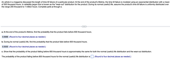
Transcribed Image Text:An article in a magazine discussed the length of time till failure of a particular product. At the end of the product's lifetime, the time till failure is modeled using an exponential distribution with a mean
of 500 thousand hours. In reliability jargon this is known as the "wear-out" distribution for the product. During its normal (useful) life, assume the product's time till failure is uniformly distributed over
the range 200 thousand to 1 million hours. Complete parts a through c.
a. At the end of the product's lifetime, find the probability that the product fails before 600 thousand hours.
0.6988 (Round to four decimal places as needed.)
b. During its normal (useful) life, find the probability that the product fails before 600 thousand hours.
0.5000 (Round to four decimal places as needed.)
c. Show that the probability of the product failing before 855 thousand hours is approximately the same for both the normal (useful) life distribution and the wear-out distribution.
The probability of the product failing before 855 thousand hours for the normal (useful) life distribution is
(Round to four decimal places as needed.)
Solution
by Bartleby Expert
Follow-up Question
Please do part b)

Transcribed Image Text:An article in a magazine discussed the length of time till failure of a particular product. At the end of the product's lifetime, the time till failure is modeled using an exponential distribution with a mean
of 500 thousand hours. In reliability jargon this is known as the "wear-out" distribution for the product. During its normal (useful) life, assume the product's time till failure is uniformly distributed over
the range 200 thousand to 1 million hours. Complete parts a through c.
a. At the end of the product's lifetime, find the probability that the product fails before 600 thousand hours.
0.6988 (Round to four decimal places as needed.)
b. During normal (useful) life, find the probability that the product fails before 600 thousand hours.
(Round to four decimal places as needed.)
Solution
by Bartleby Expert
Follow-up Questions
Read through expert solutions to related follow-up questions below.
Follow-up Question
Please do part c)

Transcribed Image Text:An article in a magazine discussed the length of time till failure of a particular product. At the end of the product's lifetime, the time till failure is modeled using an exponential distribution with a mean
of 500 thousand hours. In reliability jargon this is known as the "wear-out" distribution for the product. During its normal (useful) life, assume the product's time till failure is uniformly distributed over
the range 200 thousand to 1 million hours. Complete parts a through c.
a. At the end of the product's lifetime, find the probability that the product fails before 600 thousand hours.
0.6988 (Round to four decimal places as needed.)
b. During its normal (useful) life, find the probability that the product fails before 600 thousand hours.
0.5000 (Round to four decimal places as needed.)
c. Show that the probability of the product failing before 855 thousand hours is approximately the same for both the normal (useful) life distribution and the wear-out distribution.
The probability of the product failing before 855 thousand hours for the normal (useful) life distribution is
(Round to four decimal places as needed.)
Solution
by Bartleby Expert
Follow-up Question
Please do part b)

Transcribed Image Text:An article in a magazine discussed the length of time till failure of a particular product. At the end of the product's lifetime, the time till failure is modeled using an exponential distribution with a mean
of 500 thousand hours. In reliability jargon this is known as the "wear-out" distribution for the product. During its normal (useful) life, assume the product's time till failure is uniformly distributed over
the range 200 thousand to 1 million hours. Complete parts a through c.
a. At the end of the product's lifetime, find the probability that the product fails before 600 thousand hours.
0.6988 (Round to four decimal places as needed.)
b. During normal (useful) life, find the probability that the product fails before 600 thousand hours.
(Round to four decimal places as needed.)
Solution
by Bartleby Expert
Knowledge Booster
Similar questions
- Researchers often rely on surveys to capture a subjective assessment of well-being. One study finds that holding everything else constant, people seem to be least happy when they are in their 40's. Another study suggests that money does buy happiness, but its effects diminishes as income rises above $75000 a year. The accompanying data file includes survey daa of 100 working adults' self-assessed happiness on a scale of ) to 100, along with their age and annual income. Estimate and interpret a regression model based on Age, Age 2 and income. Predict happiness with income equal = to $80000 and age equal to 30, 45, and 60 Years Predict happiness with Age equal = to 60 and income equal to 25,000, 75000, and 125000 Happiness Age Income 69 49 52000 83 47 123000 86 72 112000 73 52 166000 89 68 90000 81 37 152000 75 48 58000 56 48 50000 75 56 93000 57 51 27000 77 60 173000 83 55 173000 85 75 68000 82 69 157000 63 39 40000 70 66 107000 78 34 109000 53…arrow_forwardIf actual period demand varies from the forecast by more than 3MAD, this indicates: there is 3% chance that the forecast is wrong. there is a 98% chance that the forecast is wrong. there is a 97% chance that the forecast is wrong. there is a 3% chance that the forecast is correct Moving to the next question prevents changes to this answer:arrow_forwardPreviously, De Anza's statistics students estimated that the amount of change daytime statistics students carry is exponentially distributed with a mean of $0.88. Suppose that we randomly pick 25 daytime statistics students. Find the probability that an individual had between $0.80 and $1.00. Graph the situation, and shade in the area to be determined.arrow_forward
- Two geysers that are near to each other are labelled as Geyser A and Geyser B. The time between eruptions for a given geyser follows an exponential distribution. The eruption times of the two geysers are independent of one another. The mean amount of time between eruptions of Geyser A is 39 minutes, and the mean amount of time between eruptions of Geyser B is 66 minutes. Given that exactly one of the geysers erupts within the next 49 minutes, determine the probability that it will be Geyser A. O 0.6654 0.7850 O 0.7252 O 0.6953 O 0.7551arrow_forwardThe numbers of polio cases in the world are shown in the table for various years. Year Number of Polio Cases (thousands) 1988 1992 1996 2000 2005 2007 350 138 33 3 3.2 1.3 Let f(t) be the number of polio cases (in thousands) t years after 1980. Copy the data to Desmos to draw a scatterplot of the data. Make sure to adjust the years so they represent years after 1980. a) Is it better to model the data with a linear or with an exponential model? [Select an answer b) Use regression in Desmos to find an appropriate model for f. Make sure to check Log mode in the parameter window in Desmos if you are fitting an exponential model. f(t) Round the coefficients to 4 decimal places. Hint: Use the variablet from the drop down menu when entering the equation. Do not just type in t. c) Predict the number of polio cases in 2013. d) Find the approximate half-life of the number of polio cases. Round the answer to one decimal place. yearsarrow_forwardPesticide danger: One of the factors that determines the degree of risk a pesticide poses to human health is the rate at which a pesticide is absorbed into skin after contact. An important question is whether the amount in the skin continues to increase with the length of the contact, or whether it increases for only a short time before leveling off. To investigate this, measured amounts of a certain pesticide were applied to 20 samples of rat skin. Four skins were analyzed at each of the time intervals 1, 2, 4, 10, and 24 hours. The amounts of the chemical (in micrograms) that were in the skin are given in the following table. Duration Amounts Absorbed 1 1.5 2.7 1.6 1.6 2 1.7 1.7 2.4 2.3 4 1.4 2.1 1.6 1.2 10 2.4 1.2 2.1 2.6 24 2.2 1.8 1.7 1.3 Send data to Excel Part: 0 / 2 Part 1 of 2 (a) Construct an ANOVA table. Round your answers to four decimal places. One-way ANOVA: Pesticide Amount Source DF SS MS F Duration Error Totalarrow_forward
arrow_back_ios
arrow_forward_ios
Recommended textbooks for you
 A First Course in Probability (10th Edition)ProbabilityISBN:9780134753119Author:Sheldon RossPublisher:PEARSON

A First Course in Probability (10th Edition)
Probability
ISBN:9780134753119
Author:Sheldon Ross
Publisher:PEARSON
