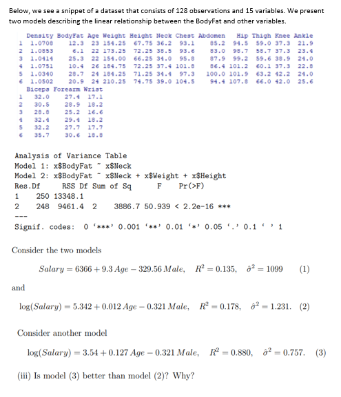
Below, we see a snippet of a dataset that consists of 128 observations and 15 variables. We present two models describing the linear relationship between the BodyFat and other variables. 2 58.7 37.3 23.4 Density BodyFat Age Weight Height Neck Chest Abdomen Hip Thigh Knee Ankle 1 1.0708 12.3 23 154.25 67.75 36.2 93.1 85.2 94.5 59.0 37.3 21.9 6.1 22 173.25 72.25 38.5 93.6 83.0 98.7 25.3 22 154.00 66.25 34.0 95.8 87.9 99.2 10.4 26 184.75 72.25 37.4 101.8 86.4 101.2 28.7 24 184.25 71.25 34.4 97.3 20.9 24 210.25 74.75 39.0 104.5 59.6 38.9 1.0853 3 1.0414 4 1.0751 5 1.0340 6 1.0502 24.0 60.1 37.3 22.8 63.2 42.2 24.0 100.0 101.9 94.4 107.8 66.0 42.0 25.6 Biceps Forearm Wrist 1 32.0 27.4 17.1 2 30.5 28.9 18.2 3 20.0 25.2 16.6 32.4 29.4 18.2 5 32.2 27.7 17.7 30.6 18.8 35.7 Analysis of Variance Table Model 1: x$BodyFat x$Neck Model 2: x$BodyFat Res. Df x$Neck + xSWeight + x$Height F Pr (>F) RSS Df Sum of Sq 1 250 13348.1 2 248 9461.4 2 3886.7 50.939 < 2.2e-16 *** Signif. codes: 0*** 0.001 **0.01 * 0.05 0.11 Consider the two models Salary = 6366 +9.3 Age-329.56 Male, R² = 0.135, ² = 1099 (1) and log(Salary) = 5.342 +0.012 Age -0.321 Male, R² = 0.178, 8²=1.231. (2) Consider another model log(Salary) = 3.54 +0.127 Age -0.321 Male, R²=0.880, 820.757. (3) (iii) Is model (3) better than model (2)? Why?

Prehistoric pottery vessels are usually found as sherds (broken pieces) and are carefully reconstructed if enough sherds can be found. Information taken from Mimbres Mogollon Archaeology by A. I. Woosley and A. J. McIntyre (University of New Mexico Press) provides data relating x = body diameter in centimeters and y = height in centimeters of prehistoric vessels reconstructed from sherds found at a prehistoric site. The following Minitab printout provides an analysis of the data. Predictor Coef SE Coef T P Constant -0.212 2.429 -0.09 0.929 Diameter 0.7527 0.1686 5.33 0.013 S = 4.16190 R-Sq = 81.2%         (c) The formula for the margin of error E for a c% confidence interval for the slope ? can be written as E = tc(SE Coef). The Minitab display is based on n = 12 data pairs. Find the critical value tc for a 90% confidence interval in the relevant table. Then find a 90% confidence interval for the population slope ?. (Use 3 decimal places.) tc   lower limit   upper…

A statistical program is recommended. A study of emergency service facilities investigated the relationship between the number of facilities and the average distance traveled to provide the emergency service. The following table gives the data collected. Average Number of Facilities Distance (miles) 1.67 11 1.11 16 0.82 21 0.62 27 0.50 30 0.47 (a) Develop a scatter diagram for these data, treating average distance traveled as the dependent variable. 1.8 1.8 35 1.8- 1.6 1.6 1.6 1.4 30 1.4 1.4 a 1.2 1.2 25 1.2 1. 1. E 1. 0.8 20 0.8 0.8- 0.6 0.6- 15 0.6- 0.4- 0.4- 0.4 0.2 10 0.2- 0. 5 0.2 10 15 20 25 30 35 0. 5 0. 10 15 20 25 30 35 0. 0.2 0.4 0.6 0.8 1. 1.2 1.4 1.6 1.8 10 15 20 25 30 35 Number Number Distance Number (b) Does a simple linear regression model appear to be appropriate? Explain. O Yes, the scatter diagram suggests that there is a linear relationship. O No, the scatter diagram suggests that there is a curvilinear relationship. O No, the scatter diagram suggests that there is…

Listed below are paired data consisting of amounts spent on advertising (in millions of dollars) and the profits (in millions of dollars). Determine if there is significant linear correlation between advertising cost and profit . Use a significance level of 0.10 and round all values to 4 decimal places. Advertising Cost Profit 3 23 4 23 5 22 6 26 7 25 8 25 9 25 10 30 11 31 12 31   Ho: ρ = 0Ha: ρ ≠ 0 Find the Linear Correlation Coefficient    r =  Find the p-value   p-value =

The weights (in pounds) of 6 vehicles and the variability of their braking distances (in feet) when stopping on a dry surface are shown in the table. Can you conclude that there is a significant linear correlation between vehicle weight and variability in braking distance on a dry surface? Use a = 0.05. Weight, x Variability in braking distance, y 5980 5370 6500 5100 5820 4800 1.72 1.97 1.87 1.63 1.64 1.50 Click here to view a table of critical values for Student's t-distribution. Setup the hypothesis for the test. Ho: Ha: P Identify the critical value(s). Select the correct choice below and fill in any answer boxes within your choice. (Round to three decimal places as needed.) O A. The critical value is. B. The critical values are - to and to %3D Calculate the test statistic. t= (Round to three decimal places as needed.) What is your conclusion? There enough evidence at the 5% level of significance to conclude that there a significant linear correlation between vehicle weight and…

Report the correlations between the three independent variables (age, educ and Protestant) and your dependent variable (childs). Which category had the correlation that was the weakest?

Q9 The explanatory variable in linear correlation/regression model is recorded on which of thesemeasurement scales: A. categorical B. ordinal C. quantitative D. none of the above

Can you please check my work

According to the February 2008 Federal Trade Commission report on consumer fraud and identity theft, 23% of all complaints in 2007 were for identity theft. In that year, assume some state had 534 complaints of identity theft out of 1960 consumer complaints. Do these data provide enough evidence to show that that state had a higher proportion of identity theft than 23%? Test at the 6% level.P: PARAMETER      What is the correct parameter symbol for this problem?                    What is the wording of the parameter in the context of this problem?              H: HYPOTHESES      Fill in the correct null and alternative hypotheses:        ASSUMPTIONS      Since     information was collected from each object, what conditions do we need to check?      Check all that apply. np≥10np≥10 n≥30n≥30 or normal population. σσ is known. σσ is unknown. N≥20nN≥20n n(1−p)≥10