
MATLAB: An Introduction with Applications
6th Edition
ISBN: 9781119256830
Author: Amos Gilat
Publisher: John Wiley & Sons Inc
expand_more
expand_more
format_list_bulleted
Related questions
Question
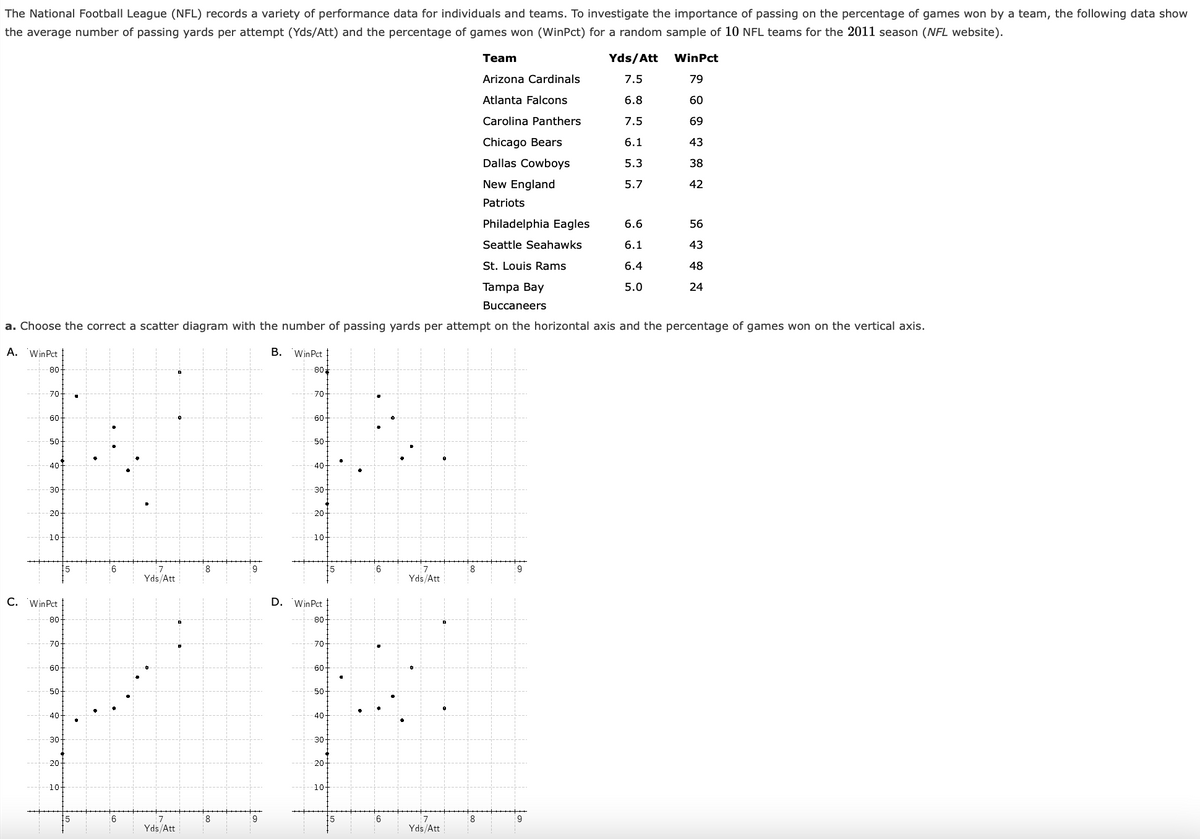

Transcribed Image Text:The National Football League (NFL) records a variety of performance data for individuals and teams. To investigate the importance of passing on the percentage of games won by a team, the following data show
the average number of passing yards per attempt (Yds/Att) and the percentage of games won (WinPct) for a random sample of 10 NFL teams for the 2011 season (NFL website).
Team
Arizona Cardinals
Atlanta Falcons
Carolina Panthers
Chicago Bears
Dallas Cowboys
New England
Patriots
Philadelphia Eagles
Seattle Seahawks
St. Louis Rams
Tampa Bay
Buccaneers
a. Choose the correct a scatter diagram with the number of passing yards per attempt on the horizontal axis and the percentage of games won on the vertical axis.
A. WinPct
80-
70+
60-
50-
30
C. WinPct
80-
70-
-60-
50-
40-
-30-
20-
6
Yds/Att
7
Yds/Att
8
9
B.
Win Pct
80
70-
60-
50+
40-
30-
D. WinPct
80-
70+
60-
50-
40-
30-
20-
6
Yds/Att
7
Yds/Att
8
9
Yds/Att
7.5
6.8
7.5
6.1
5.3
5.7
6.6
6.1
6.4
5.0
WinPct
79
60
69
43
38
42
56
43
48
24

Transcribed Image Text:b. What does the scatter diagram developed in part (a) indicate about the relationship between the two variables?
The scatter diagram indicates a positive
linear relationship between x = average number of passing yards per attempt and y = the percentage of games won by the team.
c. Develop the estimated regression equation that could be used to predict the percentage of games won given the average number of passing yards per attempt. Enter negative value as negative number.
WinPct =
* +(
) (Yds/Att) (to 4 decimals)
d. Provide an interpretation for the slope of the estimated regression equation (to 1 decimal).
So, for every increase
The slope of the estimated regression line is approximately
team increases by
*%.
✔ of one yard in the average number of passes per attempt, the percentage of games won by the
e. For the 2011 season, the average number of passing yards per attempt for the Kansas City Chiefs was was 6.5. Use the estimated regression equation developed in part (c) to predict the percentage of games
won by the Kansas City Chiefs. (Note: For the 2011 season the Kansas City Chiefs' record was wins and 9 losses.)
% (to 2 decimals)
Compare your prediction to the actual percentage of games won by the Kansas City Chiefs.
Considering the small data size, the prediction made using the estimated regression equation is not too bad
Expert Solution
This question has been solved!
Explore an expertly crafted, step-by-step solution for a thorough understanding of key concepts.

This is a popular solution

Trending nowThis is a popular solution!

Step by stepSolved in 3 steps with 2 images

Knowledge Booster

Similar questions
- A trucking company considered a multiple regression model for relating the dependent variable y = total daily travel time for one of its drivers (hours) to the predictors x₁ = distance traveled (miles) and x₂ = the number of deliveries made. Suppose that the model equation is Y = -0.800+ 0.060x₁ +0.900x₂ + e (a) What is the mean value of travel time when distance traveled is 50 miles and four deliveries are made? hr (b) How would you interpret ₁ = 0.060, the coefficient of the predictor x₁? O When the number of deliveries is constant, the average change in travel time associated with a ten-mile (i.e. one unit) increase in distance traveled is 0.060 hours. O The total daily travel time increases by 0.060 hours when the distance traveled increases by 1. O When the number of deliveries is held fixed, the average change in travel time associated with a one-mile (i.e. one unit) increase in distance traveled is 0.060 hours. O The average change in travel time associated with a one-mile (i.e.…arrow_forwardAriel was running analyses over and over in census data and came across a correlation between weight and debt (r=.78). Independent variable is weight and dependent variable is debt. b) Curious Ariel noted some statistics on these weight (M=160lb, SD=15lb) and debt (M=196k, SD=20k). If Ariel wanted to calculate a regression equation, what would her slope and intercept be?arrow_forwardWrite out the regression equation based on the output. What happens to exam performance with every increase in exam anxiety and what do you notice about the standardized regression coefficient (Beta) and the correlation?arrow_forward
- The accompanying table shows results from regressions performed on data from a random sample of 21 cars. The response (y) variable is CITY (fuel consumption in mi/gal). The predictor (x) variables are WT (weight in pounds), DISP (engine displacement in liters), and HWY (highway fuel consumption in mi/gal). The equation CITY - 3.17 +0.823HWY was previously determined to be the best for predicting city fuel consumption. A car weighs 2700 lb, it has an engine displacement of 1.6 L, and its highway fuel consumption is 35 mi/gal. What is the best predicted value of the city fuel consumption? Is that predicted value likely to be a good estimate? Is that predicted value likely to be very accurate? Click the icon to view the table of regression equations. The best predicted value of the city fuel consumption is (Type an integer or a decimal. Do not round.). Regression Table I R² Adjusted R2 WT/DISP WT/HWY Predictor (x) Variables P-Value WT/DISP/HWY 0.000 0.942 0.000 0.748 0.000 0.942 0.000…arrow_forwardB b. What does the scatter diagram developed in part (a) indicate about the relationship between the two variables? The scatter diagram indicates a positive linear relationship between a = average number of passing yar and y = the percentage of games won by the team. c. Develop the estimated regression equation that could be used to predict the percentage of games won given the avera passing yards per attempt. Enter negative value as negative number. WinPct =| |)(Yds/Att) (to 4 decimals) d. Provide an interpretation for the slope of the estimated regression equation (to 1 decimal). The slope of the estimated regression line is approximately So, for every increase : of one yar number of passes per attempt, the percentage of games won by the team increases by %. e. For the 2011 season, the average number of passing yards per attempt for the Kansas City Chiefs was was 5.5. Use th regression equation developed in part (c) to predict the percentage of games won by the Kansas City Chiefs.…arrow_forwardFor 39 nations, a correlation of 0.887 was found between y = Internet use (%) and x = gross domestic product (GDP, in thousands of dollars per capita). The regression equation is y = -3.68 + 1.73x. Complete parts (a) through (c). a. Based on the correlation value, the slope had to be positive. Why? A. The slope and correlation are positive because gross domestic product could not be negative. B. The correlation and the slope are positive because the y-intercept is negative. C. That is a very unusual fact, because the slope and correlation usually have different signs. D. Although slope and correlation usually have different values, they always have the same sign.arrow_forward
arrow_back_ios
arrow_forward_ios
Recommended textbooks for you
- MATLAB: An Introduction with ApplicationsStatisticsISBN:9781119256830Author:Amos GilatPublisher:John Wiley & Sons Inc
 Probability and Statistics for Engineering and th...StatisticsISBN:9781305251809Author:Jay L. DevorePublisher:Cengage Learning
 Statistics for The Behavioral Sciences (MindTap C...StatisticsISBN:9781305504912Author:Frederick J Gravetter, Larry B. WallnauPublisher:Cengage Learning
  Elementary Statistics: Picturing the World (7th E...StatisticsISBN:9780134683416Author:Ron Larson, Betsy FarberPublisher:PEARSON
 The Basic Practice of StatisticsStatisticsISBN:9781319042578Author:David S. Moore, William I. Notz, Michael A. FlignerPublisher:W. H. Freeman
 Introduction to the Practice of StatisticsStatisticsISBN:9781319013387Author:David S. Moore, George P. McCabe, Bruce A. CraigPublisher:W. H. Freeman
MATLAB: An Introduction with Applications
Statistics
ISBN:9781119256830
Author:Amos Gilat
Publisher:John Wiley & Sons Inc
Probability and Statistics for Engineering and th...
Statistics
ISBN:9781305251809
Author:Jay L. Devore
Publisher:Cengage Learning
Statistics for The Behavioral Sciences (MindTap C...
Statistics
ISBN:9781305504912
Author:Frederick J Gravetter, Larry B. Wallnau
Publisher:Cengage Learning
Elementary Statistics: Picturing the World (7th E...
Statistics
ISBN:9780134683416
Author:Ron Larson, Betsy Farber
Publisher:PEARSON
The Basic Practice of Statistics
Statistics
ISBN:9781319042578
Author:David S. Moore, William I. Notz, Michael A. Fligner
Publisher:W. H. Freeman
Introduction to the Practice of Statistics
Statistics
ISBN:9781319013387
Author:David S. Moore, George P. McCabe, Bruce A. Craig
Publisher:W. H. Freeman