A First Course in Probability (10th Edition)
10th Edition
ISBN: 9780134753119
Author: Sheldon Ross
Publisher: PEARSON
expand_more
expand_more
format_list_bulleted
Question

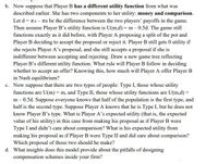
Transcribed Image Text:b. Now suppose that Player B has a different utility function from what was
described earlier. She has two components to her utility: money and comparison.
Let d = TA – TB be the difference between the two players' payoffs in the game.
Then assume Player B's utility function is U(m,d) = m – 0.5d. The game still
functions exactly as it did before, with Player A proposing a split of the pot and
Player B deciding to accept the proposal or reject it. Player B still gets 0 utility if
she rejects Player A's proposal, and she still accepts a proposal if she is
indifferent between accepting and rejecting. Draw a new game tree reflecting
Player B's different utility function. What rule will Player B follow in deciding
whether to accept an offer? Knowing this, how much will Player A offer Player B
in Nash equilibrium?
c. Now suppose that there are two types of people: Type I, those whose utility
functions are U(m) = m, and Type II, those whose utility functions are U(m,d) =
m- 0.5d. Suppose everyone knows that half of the population is the first type, and
half is the second type. Suppose Player A knows that he is Type I, but he does not
know Player B's type. What is Player A's expected utility (that is, the expected
value of his utility) in this case from making his proposal as if Player B were
Type I and didn't care about comparison? What is his expected utility from
making his proposal as if Player B were Type II and did care about comparison?
Which proposal of those two should he make?
d. What insights does this model provide about the pitfalls of designing
compensation schemes inside your firm?

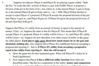
Transcribed Image Text:3.
Suppose two players, Player A and Player B, are playing a game called, "Split
the Pot." It works like this: in front of them is a pot with $1000. Player A proposes a
division of the pot in the form of (TA, TB), where TA is the amount Player A gets to keep,
TB is the amount Player B gets to keep, and TA + TB = 1000. Player B then decides to
accept or reject Player A's proposal. If Player B accepts the proposed division of the pot,
then Player A gets TA, and Player B gets TB. If Player B rejects the proposed division of
the pot, then they both get 0.
Suppose that Player A's utility from an amount of money is equal to the amount of
money: U(m) = m. Suppose the same is true for Player B. This means that if Player B
accepts Player A's proposal, Player A's utility will be U(TA) = TA, and Player B's utility
will be U(TB) = TB. Suppose for now that there is no other source of utility in this game
for either player. Each player only cares about how much money he or she gets and
absolutely nothing else. Also suppose that if Player B is indifferent between accepting a
proposal and rejecting it – that is, if Player B's utility from accepting a proposal is
equal to her utility from rejecting it – then she will accept it.
a. Draw the game tree for this sequential game. What will Player B's utility be in
Nash Equilibrium?
b. Now suppose that Player B has a different utility function from what was
described earlier. She has two components to her utility: money and comparison.
Lot d-
be the difforon0e hotwoon the
vors' no uoff. in the
Expert Solution
This question has been solved!
Explore an expertly crafted, step-by-step solution for a thorough understanding of key concepts.
This is a popular solution
Trending nowThis is a popular solution!
Step by stepSolved in 2 steps with 1 images

Knowledge Booster
Similar questions
- You are part of a government task force evaluating whether new models of cars will meet fuel efficiency standards set out by the newly signed climate bill. You have run an ANCOVA model that predicts fuel efficiency (in miles per gallon) as a function of vehicle weight (measured in thousands of lbs, where a value of 2.5 would correspond to 2,500 lbs), horsepower, and number of cylinders in the car (cylinders is a factor in this model with 3 levels: 4 cylinders, 6 cylinders, and 8 cylinders). Your analysis tells you the following; The mean miles per gallon of all cars analyzed is 20.09 The mean weight of all cars analyzed is 3.217 thousand lbs The mean horsepower of all cars analyzed is 146.7 The regression coefficient for weight is -3.18 miles per gallon per additional thousand lbs The regression coefficient for horsepower is -0.023 miles per gallon per additional unit of horsepower Cars with 4 cylinders get 2.13 more miles per gallon, on average, than the average car Toyota is…arrow_forward30 QUESTION 14 Question 9. (CUSTOMERS ARE ASSESTS FOR A BUSINESS) A saleswoman buys the five products say, bag, sunglass, watch, makeup set, and fountain pen from a supplier. Let x = 78, x2 = 25, x3 = 22, x4 = 40 and x5 =10 be the costs respectively. A saleswoman sets a profit of $3 at the end of day from the five items. If she sold two items of each product, compute her total sale as: 5 2 Σx +3 i=1 QUESTION 15arrow_forwardA company manufactures two products. If it charges price pi for product i, it can sell qi units of product i, where q1 = 80 – 2p1 + p2 and q2 = 100 – 3p2 + p1. It costs $8 to produce a unit of product 1 and $15 to produce a unit of product 2. a. How many units of each product should the company produce to maximize its profit? If needed, round your answers to one decimal digit. Product 1 Product 2 Production quantities b. What prices should the company charge to maximize its profit? If needed, round your answers to the nearest cent. Product 1 Product 2 Prices $ $arrow_forward
- Which model appears to be the best accordingly? A. Model I B. Model II C. Model III D. Model IVarrow_forwardA researcher wishes to examine the relationship between years of schooling completed and the number of pregnancies in young women. Her research discovers a linear relationship, and the least squares line is: ŷ = 2 – 3x where x is the number of years of schooling completed and y is the number of pregnancies. The slope of the regression line can be interpreted in the following way: O When amount of schooling increases by one year, the number of pregnancies tends to decrease by 2. O When amount of schooling increases by one year, the number of pregnancies tends to increase by 3. O When amount of schooling increases by one year, the number of pregnancies tends to decrease by 3. O When amount of schooling increases by one year, the number of pregnancies tends to increase by 2.arrow_forwardPlease explain the answer alongside the steps. Thank you!arrow_forward
- A restaurant is working to determine the supply and demand for their newest entrée. Based on preliminary research, they found that their demand function is 5q+28p=962 and the supply function is -q+7p=47 p q is the number of entrées ordered. Based on their preliminary research, what would be the market equilibrium price for the new entrée?arrow_forwardA researcher wishes to examine the relationship between years of schooling completed and the number of pregnancies in young women. Her research discovers a linear relationship, and the least squares line is: ŷ = 2 – 3xwhere x is the number of years of schooling completed and y is the number of pregnancies. The slope of the regression line can be interpreted in the following way: %3D O When amount of schooling increases by one year, the number of pregnancies decreases by 2. O When amount of schooling increases by one year, the number of pregnancies increases by 2. O When amount of schooling increases by one year, the number of pregnancies decreases by 3. O When amount of schooling increases by one year, the number of pregnancies increases by 3.arrow_forwardA researcher wishes to examine the relationship between years of schooling completed and the number of pregnancies in young women. Her research discovers a linear relationship, and the least squares line is: ŷ = 25x where x is the number of years of schooling completed and y is the number of pregnancies. The slope of the regression line can be interpreted in the following way: When amount of schooling increases by one year, the number of pregnancies tends to increase by 5. When amount of schooling increases by one year, the number of pregnancies tends to decrease by 5. When amount of schooling increases by one year, the number of pregnancies tends to increase by 2. When amount of schooling increases by one year, the number of pregnancies tends to decrease by 2.arrow_forward
- A researcher wishes to examine the relationship between years of schooling completed and the number of pregnancies in young women. Her research discovers a linear relationship, and the least squares line is: ˆy=3−5x where x is the number of years of schooling completed and y is the number of pregnancies. The slope of the regression line can be interpreted in the following way: When amount of schooling increases by one year, the number of pregnancies tends to decrease by 3. When amount of schooling increases by one year, the number of pregnancies tends to decrease by 5. When amount of schooling increases by one year, the number of pregnancies tends to increase by 5. When amount of schooling increases by one year, the number of pregnancies tends to increase by 3.arrow_forwardConsider the following model of a market for a good, in which Qs is quantity produced, Qd is quantity purchased and P is the price of the good. Qs=j+kP Qd=l-mP Assume that j=10, k=1, l=50, m=3. When Qs=Qd what will the price be? a. 15 b. 12 c. 10 d. 20arrow_forward#4arrow_forward
arrow_back_ios
SEE MORE QUESTIONS
arrow_forward_ios
Recommended textbooks for you
 A First Course in Probability (10th Edition)ProbabilityISBN:9780134753119Author:Sheldon RossPublisher:PEARSON

A First Course in Probability (10th Edition)
Probability
ISBN:9780134753119
Author:Sheldon Ross
Publisher:PEARSON
