
MATLAB: An Introduction with Applications
6th Edition
ISBN: 9781119256830
Author: Amos Gilat
Publisher: John Wiley & Sons Inc
expand_more
expand_more
format_list_bulleted
Related questions
Question
thumb_up100%
hey for that table we were supposed to answer this questions. its in the image 2. for that image there is a question which is question 6. how would you do that question please.
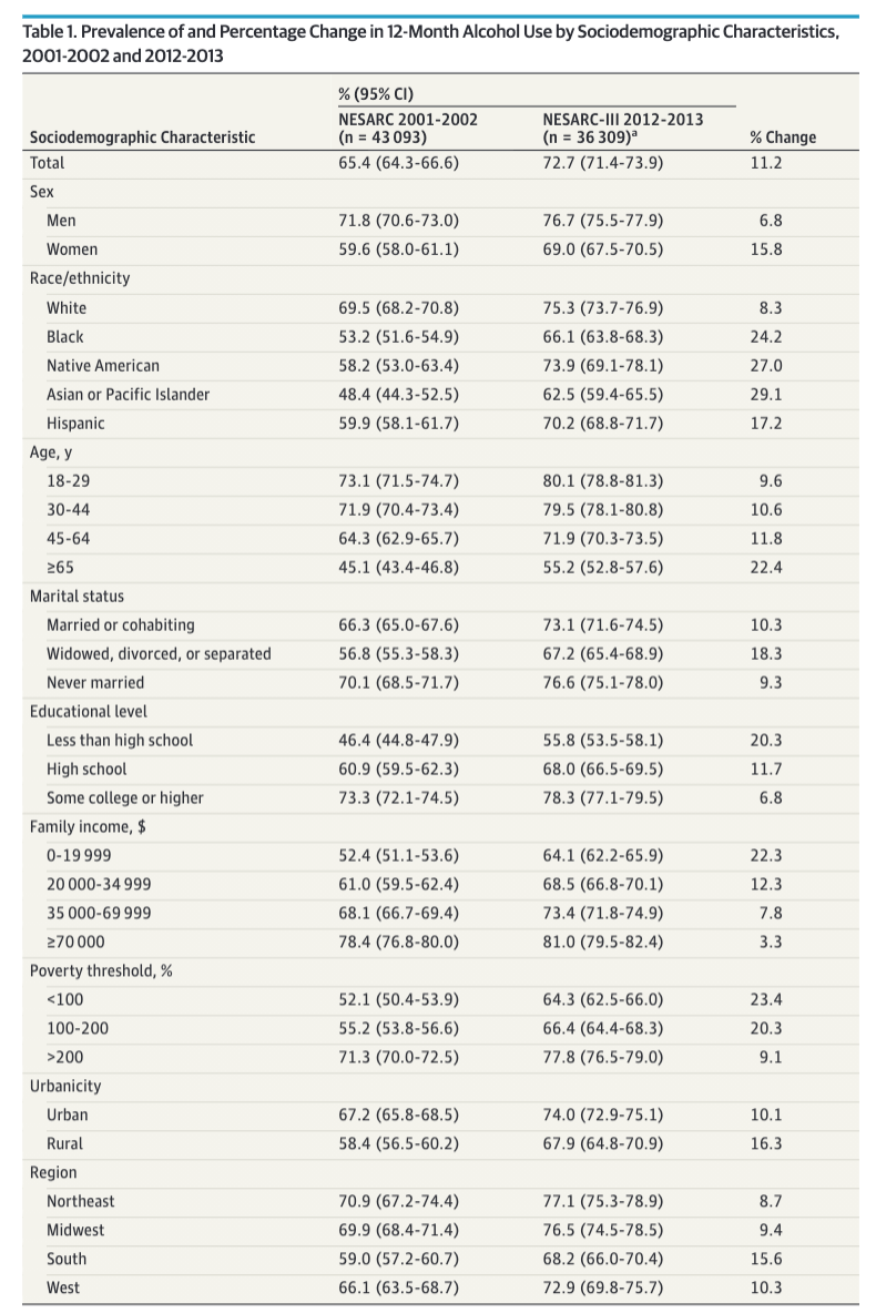

Transcribed Image Text:Table 1. Prevalence of and Percentage Change in 12-Month Alcohol Use by Sociodemographic Characteristics,
2001-2002 and 2012-2013
% (95% CI)
NESARC 2001-2002
NESARC-III 2012-2013
Sociodemographic Characteristic
(n = 43 093)
(n = 36 309)a
% Change
Total
65.4 (64.3-66.6)
72.7 (71.4-73.9)
11.2
Sex
Men
71.8 (70.6-73.0)
76.7 (75.5-77.9)
6.8
Women
59.6 (58.0-61.1)
69.0 (67.5-70.5)
15.8
Race/ethnicity
White
69.5 (68.2-70.8)
75.3 (73.7-76.9)
8.3
Black
53.2 (51.6-54.9)
66.1 (63.8-68.3)
24.2
Native American
58.2 (53.0-63.4)
73.9 (69.1-78.1)
27.0
Asian or Pacific Islander
48.4 (44.3-52.5)
62.5 (59.4-65.5)
29.1
Hispanic
59.9 (58.1-61.7)
70.2 (68.8-71.7)
17.2
Age, y
18-29
73.1 (71.5-74.7)
80.1 (78.8-81.3)
9.6
30-44
71.9 (70.4-73.4)
79.5 (78.1-80.8)
10.6
45-64
64.3 (62.9-65.7)
71.9 (70.3-73.5)
11.8
265
45.1 (43.4-46.8)
55.2 (52.8-57.6)
22.4
Marital status
Married or cohabiting
66.3 (65.0-67.6)
73.1 (71.6-74.5)
10.3
Widowed, divorced, or separated
56.8 (55.3-58.3)
67.2 (65.4-68.9)
18.3
Never married
70.1 (68.5-71.7)
76.6 (75.1-78.0)
9.3
Educational level
Less than high school
46.4 (44.8-47.9)
55.8 (53.5-58.1)
20.3
High school
60.9 (59.5-62.3)
68.0 (66.5-69.5)
11.7
Some college or higher
73.3 (72.1-74.5)
78.3 (77.1-79.5)
6.8
Family income, $
0-19 999
52.4 (51.1-53.6)
64.1 (62.2-65.9)
22.3
20 000-34 999
61.0 (59.5-62.4)
68.5 (66.8-70.1)
12.3
35 000-69 999
68.1 (66.7-69.4)
73.4 (71.8-74.9)
7.8
270000
78.4 (76.8-80.0)
81.0 (79.5-82.4)
3.3
Poverty threshold, %
<100
52.1 (50.4-53.9)
64.3 (62.5-66.0)
23.4
100-200
55.2 (53.8-56.6)
66.4 (64.4-68.3)
20.3
>200
71.3 (70.0-72.5)
77.8 (76.5-79.0)
9.1
Urbanicity
Urban
67.2 (65.8-68.5)
74.0 (72.9-75.1)
10.1
Rural
58.4 (56.5-60.2)
67.9 (64.8-70.9)
16.3
Region
Northeast
70.9 (67.2-74.4)
77.1 (75.3-78.9)
8.7
Midwest
69.9 (68.4-71.4)
76.5 (74.5-78.5)
9.4
South
59.0 (57.2-60.7)
68.2 (66.0-70.4)
15.6
West
66.1 (63.5-68.7)
72.9 (69.8-75.7)
10.3

Transcribed Image Text:What are the null and alternative
hypotheses to test if the proportion of
White Americans with 12 month
Alcohol use is different in 2012
4
1
Ho:p=
0:p = 69.5
H.
a :p > 69.5
compared to 2000?
The table says there is an 8% change Increase/ original number x 100 =
n the proportion for White Americans. þroportion
Demonstrate how this was calculated.
1
(75.3-69.5)/ 69.5 x 100 = 8.3%
Assume that the samples were
actually only 100 in each case,
calculate the relevant test statistic for
the test in part 4 above. Estimate the
þ-value. Would you Reject H,?
1
P-value:
Alternative Hypothesis is 69.5% or 0.695
The corresponding probability based on the
z-table is 0.5.
Therefore, the p-value is 1 - 0.5 = 0.5
Since p-value is > significance level, we do
hot reject H.
^ this doesn't account for the sample of
100 im not sure how to do it
LO
CO
Expert Solution
This question has been solved!
Explore an expertly crafted, step-by-step solution for a thorough understanding of key concepts.

Step by stepSolved in 2 steps

Knowledge Booster


Learn more about
Need a deep-dive on the concept behind this application? Look no further. Learn more about this topic, statistics and related others by exploring similar questions and additional content below.Similar questions
- I have two blanks to answer, what would i be putting? I'm sorry I'm confused.arrow_forwardY= -2 y=4x+6arrow_forwardTerry has taken 4 of the 5 required tests for her math class. Her grades are 83, 78, 64, and 91. Terry wants to earn at least a “B” for the course. If 80 is the minimum B grade, what is the minimum score Terry must get on her last test to get a B?arrow_forward
- The following is known about three numbers: Three times the first number plus the second number plus twice the third number is 5. If 3 times the second number is subtracted from the sum of the first number and 3 times the third number, the result is 2. If the third number is subtracted from 2 times the first number and 3 times the second number,the result is 1.(b) Find the numbers using ??????′? ?????arrow_forwardDifferentiate.arrow_forward(2,2) Lies. 6. ys-2 7. 4x +arrow_forward
- The answer is not clear this question has 4 options to pick fromarrow_forwardFirst picture is the problem and second question is the question to the problem. Please state answer from the drop down choices.arrow_forward3) Use y = -x + 5 to fill in the missing ordered pairs on the table below. y 8 10 -4 5 2.arrow_forward
arrow_back_ios
arrow_forward_ios
Recommended textbooks for you
- MATLAB: An Introduction with ApplicationsStatisticsISBN:9781119256830Author:Amos GilatPublisher:John Wiley & Sons Inc
 Probability and Statistics for Engineering and th...StatisticsISBN:9781305251809Author:Jay L. DevorePublisher:Cengage Learning
 Statistics for The Behavioral Sciences (MindTap C...StatisticsISBN:9781305504912Author:Frederick J Gravetter, Larry B. WallnauPublisher:Cengage Learning
  Elementary Statistics: Picturing the World (7th E...StatisticsISBN:9780134683416Author:Ron Larson, Betsy FarberPublisher:PEARSON
 The Basic Practice of StatisticsStatisticsISBN:9781319042578Author:David S. Moore, William I. Notz, Michael A. FlignerPublisher:W. H. Freeman
 Introduction to the Practice of StatisticsStatisticsISBN:9781319013387Author:David S. Moore, George P. McCabe, Bruce A. CraigPublisher:W. H. Freeman
MATLAB: An Introduction with Applications
Statistics
ISBN:9781119256830
Author:Amos Gilat
Publisher:John Wiley & Sons Inc
Probability and Statistics for Engineering and th...
Statistics
ISBN:9781305251809
Author:Jay L. Devore
Publisher:Cengage Learning
Statistics for The Behavioral Sciences (MindTap C...
Statistics
ISBN:9781305504912
Author:Frederick J Gravetter, Larry B. Wallnau
Publisher:Cengage Learning
Elementary Statistics: Picturing the World (7th E...
Statistics
ISBN:9780134683416
Author:Ron Larson, Betsy Farber
Publisher:PEARSON
The Basic Practice of Statistics
Statistics
ISBN:9781319042578
Author:David S. Moore, William I. Notz, Michael A. Fligner
Publisher:W. H. Freeman
Introduction to the Practice of Statistics
Statistics
ISBN:9781319013387
Author:David S. Moore, George P. McCabe, Bruce A. Craig
Publisher:W. H. Freeman