An article gave a scatter plot along with the least squares line of x = rainfall volume (m3) and y = runoff volume (m3) for a particular location. The accompanying values were read from the plot.x8121416233040515567728196112127y410131515252745384653678299102(a) Does a scatter plot of the data support the use of the simple linear regression model?Yes, the scatterplot shows a reasonable linear relationship. Yes, the scatterplot shows a random scattering with no pattern. No, the scatterplot shows a reasonable linear relationship. No, the scatterplot shows a random scattering with no pattern.(b) Calculate point estimates of the slope and intercept of the population regression line. (Round your answers to four decimal places.)slope intercept (c) Calculate a point estimate of the true average runoff volume when rainfall volume is 55. (Round your answer to four decimal places.)m3(d) Calculate a point estimate of the standard deviation ?. (Round your answer to two decimal places.)m3(e) What proportion of the observed variation in runoff volume can be attributed to the simple linear regression relationship between runoff and rainfall? 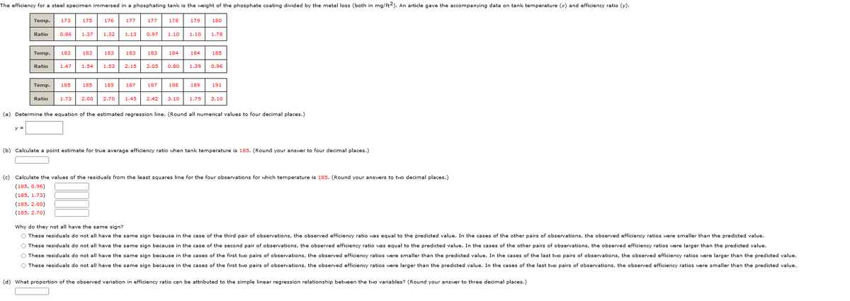(Round your answer to four decimal places.) The efficiency for a steel specimen immersed in a phosphating tank is the weight of the phosphate coating divided by the metal loss (both in mg/ft2). An article gave the accompanying data on tank temperature (x) and efficiency ratio (y).Temp. 173y =Ratio0.86Temp. 185Ratio175Temp. 183Ratio 1.47 1.541.37 1.321831761851831771851831.53 2.151.13 0.97 1.10177187178183184179187 1881801.10 1.78184 1852.05 0.80 1.39 0.961891911.73 2.00 2.70 1.45 2.42 3.10 1.79 3.10(a) Determine the equation of the estimated regression line. (Round all numerical values to four decimal places.)(b) Calculate a point estimate for true average efficiency ratio when tank temperature is 185. (Round your answer to four decimal places.)(c) Calculate the values of the residuals from the least squares line for the four observations for which temperature is 185. (Round your answers to two decimal places.)(185, 0.96)(185, 1.73)(185, 2.00)(185, 2.70)Why do they not all have the same sign?O These residuals do not all have the same sign because in the case of the third pair of observations, the observed efficiency ratio was equal to the predicted value. In the cases of the other pairs of observations, the observed efficiency ratios were smaller than the predicted value.O These residuals do not all have the same sign because in the case of the second pair of observations, the observed efficiency ratio was equal to the predicted value. In the cases of the other pairs of observations, the observed efficiency ratios were larger than the predicted value.O These residuals do not all have the same sign because in the cases of the first two pairs of observations, the observed efficiency ratios were smaller than the predicted value. In the cases of the last two pairs of observations, the observed efficiency ratios were larger than the predicted value.O These residuals do not all have the same sign because in the cases of the first two pairs of observations, the observed efficiency ratios were larger than the predicted value. In the cases of the last two pairs of observations, the observed efficiency ratios were smaller than the predicted value.(d) What proportion of the observed variation in efficiency ratio can be attributed to the simple linear regression relationship between the two variables? (Round your answer to three decimal places.)

Note: Hi there! Thank you for posting the question. As there are several independent questions with…

An article gave a scatter plot along with the least squares line of x = rainfall volume (m3) and y = runoff volume (m3) for a particular location. The accompanying values were read from the plot. x 8 12 14 16 23 30 40 51 55 67 72 81 96 112 127 y 4 10 13 15 15 25 27 45 38 46 53 67 82 99 102 (a) Does a scatter plot of the data support the use of the simple linear regression model? Yes, the scatterplot shows a reasonable linear relationship. Yes, the scatterplot shows a random scattering with no pattern. No, the scatterplot shows a reasonable linear relationship. No, the scatterplot shows a random scattering with no pattern. (b) Calculate point estimates of the slope and intercept of the population regression line. (Round your answers to four decimal places.) slope intercept (c) Calculate a point estimate of the true average runoff volume when rainfall volume is 55. (Round your answer to four decimal places.) m3 (d) Calculate a point estimate of the standard deviation ?. (Round your answer to two decimal places.) m3 (e) What proportion of the observed variation in runoff volume can be attributed to the simple linear regression relationship between runoff and rainfall? (Round your answer to four decimal places.)

6th Edition

ISBN:9781119256830

Author:Amos Gilat

Publisher:Amos Gilat

Chapter1: Starting With Matlab

Section: Chapter Questions

Problem 1P

x	8	12	14	16	23	30	40	51	55	67	72	81	96	112	127
y	4	10	13	15	15	25	27	45	38	46	53	67	82	99	102

x	8	12	14	16	23	30	40	51	55	67	72	81	96	112	127
y	4	10	13	15	15	25	27	45	38	46	53	67	82	99	102

x	8	12	14	16	23	30	40	51	55	67	72	81	96	112	127
y	4	10	13	15	15	25	27	45	38	46	53	67	82	99	102