
MATLAB: An Introduction with Applications
6th Edition
ISBN: 9781119256830
Author: Amos Gilat
Publisher: John Wiley & Sons Inc
expand_more
expand_more
format_list_bulleted
Related questions
Question
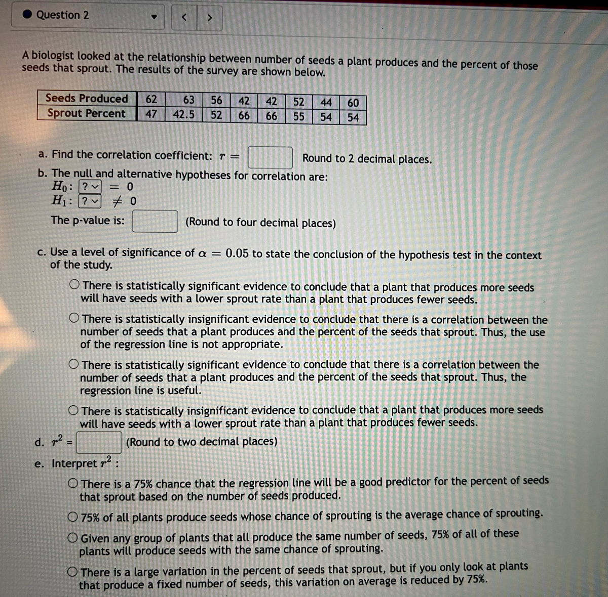

Transcribed Image Text:Question 2
<
Seeds Produced 62
Sprout Percent 47
>
A biologist looked at the relationship between number of seeds a plant produces and the percent of those
seeds that sprout. The results of the survey are shown below.
63 56 42 42 52 44 60
42.5 52 66 66
55 54 54
a. Find the correlation coefficient: r =
b. The null and alternative hypotheses for correlation are:
Ho: ?
= 0
H₁: ?0
The p-value is:
Round to 2 decimal places.
(Round to four decimal places)
c. Use a level of significance of a = 0.05 to state the conclusion of the hypothesis test in the context
of the study.
O There is statistically significant evidence to conclude that a plant that produces more seeds
will have seeds with a lower sprout rate than a plant that produces fewer seeds.
There is statistically insignificant evidence to conclude that there is a correlation between the
number of seeds that a plant produces and the percent of the seeds that sprout. Thus, the use
of the regression line is not appropriate.
O There is statistically significant evidence to conclude that there is a correlation between the
number of seeds that a plant produces and the percent of the seeds that sprout. Thus, the
regression line is useful.
There is statistically insignificant evidence to conclude that a plant that produces more seeds
will have seeds with a lower sprout rate than a plant that produces fewer seeds.
(Round to two decimal places)
d. ² =
e. Interpret ²:
O There is a 75% chance that the regression line will be a good predictor for the percent of seeds
that sprout based on the number of seeds produced.
O 75% of all plants produce seeds whose chance of sprouting is the average chance of sprouting.
O Given any group of plants that all produce the same number of seeds, 75% of all of these
plants will produce seeds with the same chance of sprouting.
O There is a large variation in the percent of seeds that sprout, but if you only look at plants
that produce a fixed number of seeds, this variation on average is reduced by 75%.

Transcribed Image Text:f. The equation of the linear regression line is:
ŷ =
+
(Please show your answers to two decimal places)
g. Use the model to predict the percent of seeds that sprout if the plant produces 51 seeds.
Percent sprouting =
(Please round your answer to the nearest whole number.)
h. Interpret the slope of the regression line in the context of the question:
O For every additional seed that a plant produces, the chance for each of the seeds to sprout
tends to decrease by 0.80 percent.
The slope has no practical meaning since it makes no sense to look at the percent of the seeds
that sprout since you cannot have a negative number.
O As x goes up, y goes down.
i. Interpret the y-intercept in the context of the question:
O If plant produces no seeds, then that plant's sprout rate will be 96.46.
The best prediction for a plant that has 0 seeds is 96.46 percent.
The y-intercept has no practical meaning for this study.
O The average sprouting percent is predicted to be 96.46.
Expert Solution
This question has been solved!
Explore an expertly crafted, step-by-step solution for a thorough understanding of key concepts.

Step by stepSolved in 6 steps with 4 images

Knowledge Booster

Similar questions
- I need help calculating the correlation coeddicient r indicating the relationship between X and Y. I need to include the necessary deviation scores and sums of squares. With that, I need to conduct a hypothesis test whether the correlation between X and Y is significant. Provide the degrees of freedom and the cut-off value, assuming a two-tailed test with alpha = 0.05. And then creating a scatterplot associated with the data.arrow_forwardDetermine whether the given correlation coefficient is statistically significant at the specified level of significance and sample size. r=−0.599 α=0.01, n=11 Yes or No?arrow_forward4. Compute the Pearson correlation for the following data. X Y 3 1 4 5 2 A researcher is interested in seeing if there is a significant relationship between the number of hours of sleep a night (X) and Productivity scores (Y). She conducts a study to test her hypothesis. Please use the data set above. a. Use a two-tailed test with a = .05. Conduct the four steps for hypothesis testing and label each step: Stepl, Step 2, Step 3, and Step 4. b. Write a sentence regarding your results. c. Calculate the regression equation for this data set. d. What are the predicted Y scores for the following X scores: X=1, X=7, X=10, X-12. 2364narrow_forward
- Four Air Force trainee pilots take a test of visual acuity (higher scores mean better acuity) and an anxiety test (higher scores mean more anxiety. The scores are as follows: Person Acuity (x) Anxiety (y) 1 1 7 2 1 8 3 2 4 4 4 -1 Calculate critical value , SP the correlation coefficient and determine whether the correlation is statistically significant at the .05 significance level, two-tailedarrow_forwardCompute the Pearson correlation for the following data.X: 2, 3, 6, 4, 5 Y :3, 1, 5, 4, 2 A researcher is interested in seeing if there is a significant relationship between the number of hours of sleep a night (X) and Productivity scores (Y). She conducts a study to test her hypothesis. Please use the data set above. Use a two-tailed test with a = 0.1. Conduct the four steps for hypothesis testing and label each step: Step1, Step 2, Step 3, and Step 4.arrow_forwardWe compute a sample correlation coefficient of r=0.692 from a set of 12 data pairs. We are testing Ho:p=0 against H;:p#0 at a = 0.05. The value of the test statistic for this test is: O 3.18 O 3.64 O 3.03 3.94arrow_forward
- Provide an interpretation for the following SPSS output: A researcher wanted to test the relationship between number of fries eaten per week and number of vegetables eaten per week by the sample. Number of times Number of times eat fries per eat vegetables week per week Number of times eat fries per Pearson Correlation 1 -.067 week Sig. (2-tailed) .005 N 1750 1750 Number of times eat Pearson Correlation -.067 1 vegetables per week Sig. (2-tailed) N .005 1750 1750 **Correlation is significant at the 0.01 level (2-tailed). Edit View Insert Format Tools Table 12pt v Paragrapharrow_forward7arrow_forwardThe accompanying table lists the ages of acting award winners matched by the years in which the awards were won. Construct a scatterplot, find the value of the linear correlation coefficient r, and find the P-value of r. Determine whether there is sufficient evidence to support a claim of linear correlation between the two variables. Should we expect that there would be a correlation? Use a significance level of = 0.05. E Click the icon to view the ages of the award winners. Construct a scatterplot. Choose the correct graph below. OA. OB. Oc. OD. 70- 70- Q 70- 70- ... ++++++ 20 - 20 Best Actress (years) 20- 70 20 Best Actress (years) 20- 20 Best Actress (years) 70 20 Best Actress (years) 70 70 Best Actresses and Best Actors Best Actress 27 29 30 58 33 34 46 30 62 22 44 51 D Best Actor 44 36 38 44 53 46 56 49 41 52 44 33arrow_forward
- a) Compute the value of the sample correlation coefficient, r. (Round your answer to four decimal places.) r = b) Calculate the test statistic and determine the P-value. (Round your test statistic to one decimal place and your P-value to three decimal places.) t = P- value = c) If a regression analysis were to be carried out to predict endurance from lactate level, what proportion of observed variation in endurance could be attributed to the approximate linear relationship? Answer the question without doing any regression calculations. (Round your answer to four decimal places.) ____________ d) If a regression analysis were to be carried out to predict lactate level from endurance, what proportion of observed variation in endurance could be attributed to the approximate linear relationship? Answer the question without doing any regression calculations. (Round your answer to four decimal places.) _____________arrow_forward(i) State the hyptheses. (ii) Sketch a scatter plot tat best represents the data. (iii) Compute the value of the correlation coefficient. Round the answer to at least three decimal places. (iv) Find the P-value. Round the answer to at least four decimal places. Test the significance of r at α=0.05. Determine whether to reject or not reject the null hypothesis.arrow_forward5.32 Fuel efficiency of manual and automatic cars, Part I: Do these data provide strong evidence of a difference between the average fuel efficiency of cars with manual and automatic transmissions in terms of their average city mileage? Assume that conditions for inference are satisfied. City MPG, Automatic City MPG, Manual Mean 16.12 19.85 SD 3.58 4.51 n 26 26 The test statistic is:The p-value is:arrow_forward
arrow_back_ios
SEE MORE QUESTIONS
arrow_forward_ios
Recommended textbooks for you
- MATLAB: An Introduction with ApplicationsStatisticsISBN:9781119256830Author:Amos GilatPublisher:John Wiley & Sons Inc
 Probability and Statistics for Engineering and th...StatisticsISBN:9781305251809Author:Jay L. DevorePublisher:Cengage Learning
 Statistics for The Behavioral Sciences (MindTap C...StatisticsISBN:9781305504912Author:Frederick J Gravetter, Larry B. WallnauPublisher:Cengage Learning
  Elementary Statistics: Picturing the World (7th E...StatisticsISBN:9780134683416Author:Ron Larson, Betsy FarberPublisher:PEARSON
 The Basic Practice of StatisticsStatisticsISBN:9781319042578Author:David S. Moore, William I. Notz, Michael A. FlignerPublisher:W. H. Freeman
 Introduction to the Practice of StatisticsStatisticsISBN:9781319013387Author:David S. Moore, George P. McCabe, Bruce A. CraigPublisher:W. H. Freeman
MATLAB: An Introduction with Applications
Statistics
ISBN:9781119256830
Author:Amos Gilat
Publisher:John Wiley & Sons Inc
Probability and Statistics for Engineering and th...
Statistics
ISBN:9781305251809
Author:Jay L. Devore
Publisher:Cengage Learning
Statistics for The Behavioral Sciences (MindTap C...
Statistics
ISBN:9781305504912
Author:Frederick J Gravetter, Larry B. Wallnau
Publisher:Cengage Learning
Elementary Statistics: Picturing the World (7th E...
Statistics
ISBN:9780134683416
Author:Ron Larson, Betsy Farber
Publisher:PEARSON
The Basic Practice of Statistics
Statistics
ISBN:9781319042578
Author:David S. Moore, William I. Notz, Michael A. Fligner
Publisher:W. H. Freeman
Introduction to the Practice of Statistics
Statistics
ISBN:9781319013387
Author:David S. Moore, George P. McCabe, Bruce A. Craig
Publisher:W. H. Freeman