Concept explainers
A physician sees many different kinds of patients, and thus the time spent with each patient varies. Let X be the time spent with a patient in minutes. From historical data, X is known to be uniformly distributed between 15 and 40 minutes.
a) What is the standard deviation of the time spent with a patient?
b) What is the likelihood that the physician will spend less than 35 minutes with a patient?
c) A patient has an appointment to see the physician at 8AM on a particular day. When should the second patient be scheduled so that there is only a 15% chance s/he will have to wait before before being seen by the physician? [e.g. if the appointment for the second patient is 8:15AM, there is a 100% chance the second patient will have to wait]
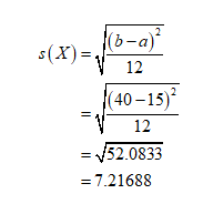
The standard deviation of the time spent with a patient can be calculated as:

Thus, the standard deviation is 7.217
Trending nowThis is a popular solution!
Step by stepSolved in 3 steps with 3 images

- The probability that a randomly chosen student in a statistics class submits his/her homework on time is 0.39. There is 46 student in the class. Each student does his/her homework independently. What is the standard deviation of X, where X is the number of students who submit the homework on time?arrow_forwardThe probability that a randomly chosen student in a statistics class submits his/her homework on time is 0.12. There is 35 student in the class. Each student does his/her homework independently. What is the standard deviation of X, where X is the number of students who submit the homework on time?arrow_forwardThe average amount of money spent for lunch per person in the college cafeteria is $6.24 and the standard deviation is $2.05. Suppose that 6 randomly selected lunch patrons are observed. Assume the distribution of money spent is normal, and round all answers to 4 decimal places where possible.What is the distribution of ¯x?arrow_forward
- Assume that final exam scores in a given course are approximately normally distributed with a mean of 75 and a standard deviation of 10 points. In a class of 200 students, how many would you expect to fail the exam (i.e., score less than 60) (note: scores can only be approximately normally distributed, because the minimum score is 0, but this should not alter the answer, given how large the mean is relative to the standard deviation).arrow_forwardPart 2. Complete the following statements. A) The cumulative enrolment is the enrolment of the intervals smaller than the interval in question or equal to the latter. The graph of cumulative enrolment is represented by a function in B) The average, median and mode are three measures of of the C) The term refers to any data that deviates disproportionately from others. D) When the residual values are zero, then the correlation is calledarrow_forwardA particular fruit's weights are normally distributed, with a mean of 455 grams and a standard deviation of 31 grams. If you pick 19 fruit at random, what is the probability that their mean weight will be between 434 grams and 443 grams? Use GeoGebra. Round to 4 places.arrow_forward
- Assume time to failure density function (in months) of transplanted kidneys has a Weibull distribution with shape factor of 3 and scale of 6. Use R and answer the following questions (enter your answers with 3 decimal points):arrow_forwardChebyshev's Theorem states that for any distribution of numerical data, at least 1-1/k? of the numbers lie within The percent of numbers between 88 and 112 is at least %. k standard deviations of the mean. (Round to the nearest hundredth as needed.) In a certain distribution of numbers, the mean is 100, with a standard deviation of 6. Use Chebyshev's Theorem to tell what percent of the numbers are between 88 and 112.arrow_forwardAssume that IQ scores are normally distributed, with a mean of 100 points and a standard deviation of 14 points. If 50 people are chosen at random, what is the probability that the sample mean of IQ scores will be between 98 and 102?P(98 ≤ x ≤ 102) = ?arrow_forward
 MATLAB: An Introduction with ApplicationsStatisticsISBN:9781119256830Author:Amos GilatPublisher:John Wiley & Sons Inc
 Probability and Statistics for Engineering and th...StatisticsISBN:9781305251809Author:Jay L. DevorePublisher:Cengage Learning
 Statistics for The Behavioral Sciences (MindTap C...StatisticsISBN:9781305504912Author:Frederick J Gravetter, Larry B. WallnauPublisher:Cengage Learning
 Elementary Statistics: Picturing the World (7th E...StatisticsISBN:9780134683416Author:Ron Larson, Betsy FarberPublisher:PEARSON
 The Basic Practice of StatisticsStatisticsISBN:9781319042578Author:David S. Moore, William I. Notz, Michael A. FlignerPublisher:W. H. Freeman
 Introduction to the Practice of StatisticsStatisticsISBN:9781319013387Author:David S. Moore, George P. McCabe, Bruce A. CraigPublisher:W. H. Freeman


