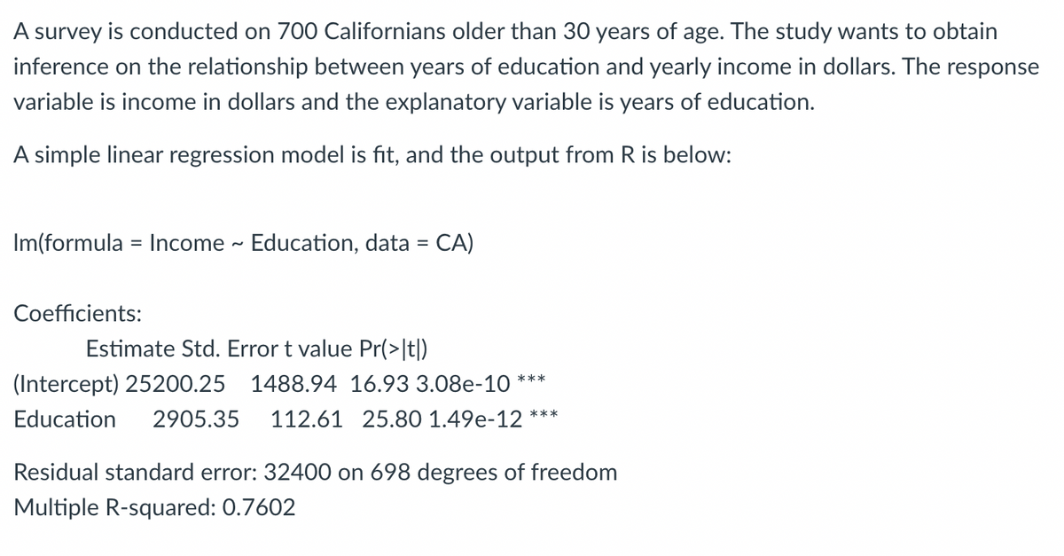
A survey is conducted on 700 Californians older than 30 years of age. The study wants to obtain inference on the relationship between years of education and yearly income in dollars. The response variable is income in dollars and the explanatory variable is years of education. A simple linear regression model is fit, and the output from R is below: Im(formula = Income ~ Education, data = CA) Coefficients: Estimate Std. Error t value Pr(>|t|) (Intercept) 25200.25 1488.94 16.93 3.08e-10 *** Education 2905.35 112.61 25.80 1.49e-12 *** Residual standard error: 32400 on 698 degrees of freedom Multiple R-squared: 0.7602

The sweetness, y, of the fruit is supposed to be related to the average daily sunshine hours, x. The following data shows the sweetness of the same type of fruit at different locations (sunshine hours). Fit the data to a simple linear regression model. x: 5, 6, 7, 6, 6, 8, 7, 5. y: 9, 10, 10, 11, 12, 13, 12, 8. Predict the true mean sweetness for average daily hours of 8 hours, and calculate the residual for average daily sunshine hours of 8 hours.

A graphing calculator is recommended. When laboratory rats are exposed to asbestos fibers, some of them develop lung tumors. The table lists the results of several experiments by different scientists. Asbestos exposure (fibers/mL) y = 50 Mice with Tumors (%) 400 O 500 900 1,100 1,600 1,800 2,000 3,000 3000 2500 2000 1500 (a) Find the regression line for the data. (Use x for asbestos exposure in fibers/mL and y for percent of mice with tumors. Round your values to four decimal places.) 1000 500 Percent of mice that develop lung tumors (b) Construct a scatter plot and graph the regression line. o 0 7 6 11 10 27 41 38 37 49 20 30 40 50 Asbestos Exposure (Fibers/mL.) 60 Mice with Tumors (%) 3000 ● 2500 2000 1500 1000 500 60 0 0 10 20 30 40 50 60 Asbestos Exposure (Fibers/mL) Ⓡ 4

The table shows a part of an output of a linear regression model predicting the average fare on different flight routes. Data Table Regression Table Coefficient Constant 95.80976147 COUPON −9.61654124 DISTANCE 0.080733811 PAX −0.000167343 What is the difference in prediction of the following two routes? Route A that is 3,000 miles, with COUPON=1.5 and PAX=6,000 Route B that is 3,000 miles, with COUPON=1.2 and PAX=6,000.

Researchers are interested in predicting the height of a child based on the heights of their mother and father. Data were collected, which included height of the child ( height), height of the mother ( mothersheight ), and height of the father (fathersheight ). The initial analysis used the heights of the parents to predict the height of the child (all units are inches). The results of the analysis, a multiple regression, are presented below. . regress height mothersheight fathersheight Source Model Residual Total height mothersheight fathersheight _cons SS 208.008457 314.295372 522.303829 df 2 104.004228 8.49446952 37 MS 39 13.3924059 Coef. Std. Err. .6579529 .1474763 .2003584 .1382237 9.804327 12.39987 t P>|t| 4.46 0.000 C 0.156 0.79 0.434 Number of obs = F( 2, 37) = Prob > F R-squared Adj R-squared = Root MSE = = .3591375 -.0797093 -15.32021 = 40 12.24 0.0001 0.3983 0.3657 2.9145 [95% Conf. Interval] .9567683 .4804261 34.92886 What are the null and alternative hypotheses…

The accompanying data are the number of wins and the earned run averages (mean number of earned runs allowed per nine innings pitched) for eight baseball pitchers in a recent season. Find the equation of the regression line. Then construct a scatter plot of the data and draw the regression line. Then use the regression equation to predict the value of y for each of the given x-values, if meaningful. If the x-value is not meaningful to predict the value of y, explain why not. (a) x = 5 wins Click the icon to view the table of numbers of wins and earned run average. (b) x = 10 wins (c) x = 21 wins (d) x = 15 wins ERA 6- ERA 6- AERA 6- ERA 6- 4- 4- 4- 4- 2- 2- 2- 2- 0+ 6 0- 0- 0- 12 18 24 6. 12 18 24 12 18 24 6 12 18 24 Wins Wins Wins Wins (a) Predict the ERA for 5 wins, if it is meaningful. Select the correct choice below and, if necessary, fill in the answer box within your choice. A. ŷ= (Round to two decimal places as needed.) B. It is not meaningful to predict this value of y because…

Using a sample of recent university graduates, you estimate a simple linear regression using initial annual salary as the dependent variable and the graduate's weighted average mark (WAM) as the explanatory variable. If the regression model has an estimated intercept of 3200 and an estimated slope coefficient of 550, what is the predicted starting salary of a student with a WAM of 64?

Find the​ least-squares regression line treating square footage as the explanatory variable.   y =  ​(Round the slope to three decimal places as needed. Round the intercept to one decimal place as​ needed.)

Pls help ASAP. Pls show all work.

The table shows the average weekly wages (in dollars) for state government employees and federal government employees for 8 years. The equation of the regression line is y = 1.405x – 12.307. Complete parts (a) and (b) below. Average Weekly Wages (state), x Average Weekly Wages (federal), y 751 760 791 817 835 881 924 951 1002 1047 1115 1149 1195 1250 1269 1300 (a) Find the coefficient of determination and interpret the result. 12 =O