
MATLAB: An Introduction with Applications
6th Edition
ISBN: 9781119256830
Author: Amos Gilat
Publisher: John Wiley & Sons Inc
expand_more
expand_more
format_list_bulleted
Related questions
Concept explainers
Question
A survey found that women's heights are
a. Find the percentage of women meeting the height requirement. Are many women being denied the opportunity to join this branch of the military because they are too short or too tall?
b. If this branch of the military changes the height requirements so that all women are eligible except the shortest 1% and the tallest 2%, what are the new height requirements?
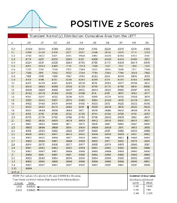

Transcribed Image Text:### Positive z Scores: Standard Normal (z) Distribution Table
#### Overview
This table displays the cumulative area from the left under the standard normal curve for positive z scores. This is useful for determining probabilities and critical values in statistical analyses.
#### Table Structure
- **Rows and Columns**: The table is organized with z scores increasing from 0.0 to 3.09 along the row headers, with additional decimals from .00 to .09 across the column headers.
- **Values**: Each cell in the table represents the cumulative probability from the left of the standard normal distribution for a given z score (intersection of row and column).
For example:
- A z score of 0.00 corresponds to a cumulative area of 0.5000.
- A z score of 1.23 corresponds to a cumulative area of 0.8907.
#### Important Calculations
- For z scores above 3.49, use 0.9999 for the cumulative area.
- **Interpolation**:
- For specific z scores like 1.645, use interpolation to find more accurate cumulative areas.
- \( z = 1.645 \) is approximately 0.9500.
- \( z = 2.575 \) is approximately 0.9950.
#### Common Critical Values
Different levels of confidence correspond to specific critical z scores:
- A 90% confidence level corresponds to a critical z value of 1.645.
- A 95% confidence level corresponds to a critical z value of 1.96.
- A 99% confidence level corresponds to a critical z value of 2.575.
#### Visual Representation
The blue bell curve diagram at the top represents the standard normal distribution. The shading under the curve indicates the area (probability) left of a specific z score.
This table is a fundamental tool in statistical data analysis, particularly for tasks involving hypothesis testing, confidence intervals, and probability calculations.

Transcribed Image Text:**Negative z-Scores**
**Standard Normal (z) Distribution: Cumulative Area from the LEFT**
This table shows the cumulative area under the standard normal curve to the left of specified z-scores, which are negative in this case. This table is used to find probabilities associated with standard normal distribution.
**z-Score Table**
- **Columns**: Represent the hundredths place of the z-score.
- **Rows**: Represent the tenths and units place of the z-score.
- **Values**: Indicate the cumulative probability to the left of the z-score.
**Example Calculations:**
- For a z-score of -3.4, use the row for -3.4 and the column for .00, resulting in a cumulative area of 0.0003.
- For a z-score of -2.57, using the interpolation, the cumulative area is approximately 0.0050.
**Graph**
The graph at the top right shows a normal distribution curve with a shaded area to the left, representing the area under the curve up to a certain z-score.
**Special Notes**
- For values of z below -3.49, use 0.0001 for the area.
- Use common values for interpolation:
- z-score: -1.645 has an area of 0.0500
- z-score: -2.575 has an area of 0.0050
This table and graph are essential for understanding probabilities in statistics, particularly those that fall below the mean in a normal distribution.
Expert Solution
This question has been solved!
Explore an expertly crafted, step-by-step solution for a thorough understanding of key concepts.

This is a popular solution

Trending nowThis is a popular solution!

Step by stepSolved in 2 steps

Knowledge Booster


Learn more about
Need a deep-dive on the concept behind this application? Look no further. Learn more about this topic, statistics and related others by exploring similar questions and additional content below.Similar questions
- ↑ The table gives the distribution on annual salanes at a small company. Use the information in the table to answer the following a) Determine the mean annual salary b) Determine the median annual salary c) Determine the mode annual salary d) Determine the midrange annual salary e) Which do you believe is the best measure of central tendency for this set of data? Explain your answer a) The mean annual salary is (Type an integer or a decimal Round to the nearest dollar as needed) Annual Number Salary Receiving Salary $105,000 $50,000 $23,000 $22.000 $19.000 $18.000 204 6 3 19arrow_forwardall parts pleasearrow_forwardA variable is normally distributed with mean 21 and standard deviation 7. Use your graphing calculator to find each of the following areas. Write your answers in decimal form. Round to the nearest thousandth as needed.a) Find the area to the left of 24. b) Find the area to the left of 15. c) Find the area to the right of 23. Incorrect d) Find the area to the right of 25. Incorrect e) Find the area between 15 and 29.arrow_forward
- A grocer finds that the cantaloupes in his store have weights with mean 0.7 kg and standard deviation 53 grams. If this is true, then 99.7% of cantaloupes will have weights between how many grams?arrow_forward1) Here are the weights in pounds of a sample of 10 students in fourth grade class: 61, 64, 66, 74, 77, 78, 78, 83, 84, 85. Find A) the mean B) standard deviationarrow_forwardCan you answer c,d, and e pleasearrow_forward
- The annual rainfall in a certain region is approximately normally distributed with mean 42.6 inches and standard deviation 5.2 inches. Round answers to the nearest tenth of a percent. a) What percentage of years will have an annual rainfall of less than 44 inches? % % b) What percentage of years will have an annual rainfall of more than 39 inches? c) What percentage of years will have an annual rainfall of between 38 inches and 43 inches? %arrow_forwardA labor rights group wants to determine the mean salary of app-based drivers. If she knows that the standard deviation is $3.3, how many drivers should she consider surveying to be 90% sure of knowing the mean will be within +$0.77? 31 O 542 33 О 50arrow_forwardThe annual rainfall in a certain region is approximately normally distributed with mean 42.5 inches and standard deviation 6 inches. Round answers to the nearest tenth of a percent.a) What percentage of years will have an annual rainfall of less than 44 inches? %b) What percentage of years will have an annual rainfall of more than 40 inches? %c) What percentage of years will have an annual rainfall of between 39 inches and 43 inches?arrow_forward
- Based on data from the 2010 Census the average age of a Pierce County, Washington resident is 41 years with a standard deviation of 12.3 . The data is normally distributed. The median age, in years, is: a) 41 b) 38 c) 43 d) 33arrow_forwardIt is generally believed that the heights of adult females in the U.S. are approximately normally distributed with mean 65 inches and standard deviation 4 inches. A small university is considering custom ordering beds for their dorm rooms. Answer the following questions about the lengths of beds in dorm rooms at this university. A. The beds that the university currently purchases are 70 inches long. What proportion of females will be able to fit on the bed while lying perfectly straight (less than 70”)? Draw/Label/Shade a curve with this information and provide the value of the requested proportion. B. What is the height of a female who is in the top 10% for her height? Draw/Label/Shadearrow_forwardConsider the numbers 1, 2, 3, 4 assigned to values of a variable. The variable being measured is most likely: a) quantitative b) qualitative c) one for which computing the standard deviation would likely be appropriate d) one for which computing the median would definitely be inappropriate e) a and carrow_forward
arrow_back_ios
arrow_forward_ios
Recommended textbooks for you
- MATLAB: An Introduction with ApplicationsStatisticsISBN:9781119256830Author:Amos GilatPublisher:John Wiley & Sons Inc
 Probability and Statistics for Engineering and th...StatisticsISBN:9781305251809Author:Jay L. DevorePublisher:Cengage Learning
 Statistics for The Behavioral Sciences (MindTap C...StatisticsISBN:9781305504912Author:Frederick J Gravetter, Larry B. WallnauPublisher:Cengage Learning
  Elementary Statistics: Picturing the World (7th E...StatisticsISBN:9780134683416Author:Ron Larson, Betsy FarberPublisher:PEARSON
 The Basic Practice of StatisticsStatisticsISBN:9781319042578Author:David S. Moore, William I. Notz, Michael A. FlignerPublisher:W. H. Freeman
 Introduction to the Practice of StatisticsStatisticsISBN:9781319013387Author:David S. Moore, George P. McCabe, Bruce A. CraigPublisher:W. H. Freeman
MATLAB: An Introduction with Applications
Statistics
ISBN:9781119256830
Author:Amos Gilat
Publisher:John Wiley & Sons Inc
Probability and Statistics for Engineering and th...
Statistics
ISBN:9781305251809
Author:Jay L. Devore
Publisher:Cengage Learning
Statistics for The Behavioral Sciences (MindTap C...
Statistics
ISBN:9781305504912
Author:Frederick J Gravetter, Larry B. Wallnau
Publisher:Cengage Learning
Elementary Statistics: Picturing the World (7th E...
Statistics
ISBN:9780134683416
Author:Ron Larson, Betsy Farber
Publisher:PEARSON
The Basic Practice of Statistics
Statistics
ISBN:9781319042578
Author:David S. Moore, William I. Notz, Michael A. Fligner
Publisher:W. H. Freeman
Introduction to the Practice of Statistics
Statistics
ISBN:9781319013387
Author:David S. Moore, George P. McCabe, Bruce A. Craig
Publisher:W. H. Freeman