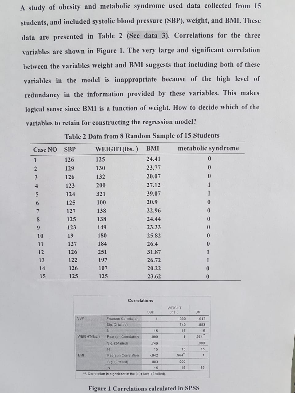
A study of obesity and metabolic syndrome used data collected from 15 students, and included systolic blood pressure (SBP), weight, and BMI. These data are presented in Table 2 (See data 3). Correlations for the three variables are shown in Figure 1. The very large and significant correlation between the variables weight and BMI suggests that including both of these variables in the model is inappropriate because of the high level of redundancy in the information provided by these variables. This makes logical sense since BMI is a function of weight. How to decide which of the variables to retain for constructing the regression model? Table 2 Data from 8 Random Sample of 15 Students Case NO SBP WEIGHT(lbs.) BMI metabolic syndrome 1 126 125 24.41 0 2 129 130 23.77 0 126 132 20.07 0 123 200 27.12 1 124 321 39.07 1 125 100 20.9 0 127 138 22.96 0 125 138 24.44 0 123 149 23.33 0 19 180 25.82 0 127 184 26.4 0 126 251 31.87 1 122 197 26.72 1 126 107 20.22 0 125 125 23.62 0 3 4 5 6 7 8 9 10 11 12 13 14 15 Correlations SBP WEIGHT (lbs.) SBP 1 Pearson Correlation Sig. (2-tailed) 15 WEIGHT(lbs.) -.090 964** N Pearson Correlation. Sig (2-tailed) N .749 .000 15 15 BMI Pearson Correlation -.042 1 Sig. (2-tailed) 883 .000 N 15 15 15 **. Correlation is significant at the 0.01 level (2-tailed). Figure 1 Comolations calaulated in SPSS -.090 749 15 1 15 BMI 964 -.042 .883 15

The condition of an independent variable being correlated to one or more other independent variables is referred to as     nonlinearity.     statistical significance.     multicollinearity.     linearity.

Fiske Corporation manufactures a popular regional brand of kitchen utensils. The design and variety has been fairly constant over the last three years. The managers at Fiske are planning for some changes in the product line next year, but first they want to understand better the relation between activity and factory costs as experienced with the current products. Discussions with the plant supervisor suggest that overhead seems to vary with labor-hours, machine-hours, or both. The following data were collected from last three year's operations: Quarter Machine-Hours 18,850 4 5 6 7 8 9 10 11 12 18,590 17,480 19,240 21,280 19,630 19,240 18,850 18,460 20,670 17,550 18,460 Labor-Hours 15,605 15,484 16,727 15,990 17,508 17,376 15,297 14,373 16,001 17,002 14,285 17,651 Factory costs $ 3,395,671 3,425,836 3,617,844 3,573,940 3,812,984 3,778,012 3,532,426 3,369,802 3,513, 187 3,731,434 3,325,615 3,724,486 Required: Prepare a scatter graph based on the factory cost and labor-hour data. Note: 1.…

The type of study that allows us to draw firm conclusions about the cause-and-effect relationship between two variables is a(n): a. experimental or quasi-experimental design b. experimental design c. correlational or quasi-experimental design d. correlational design