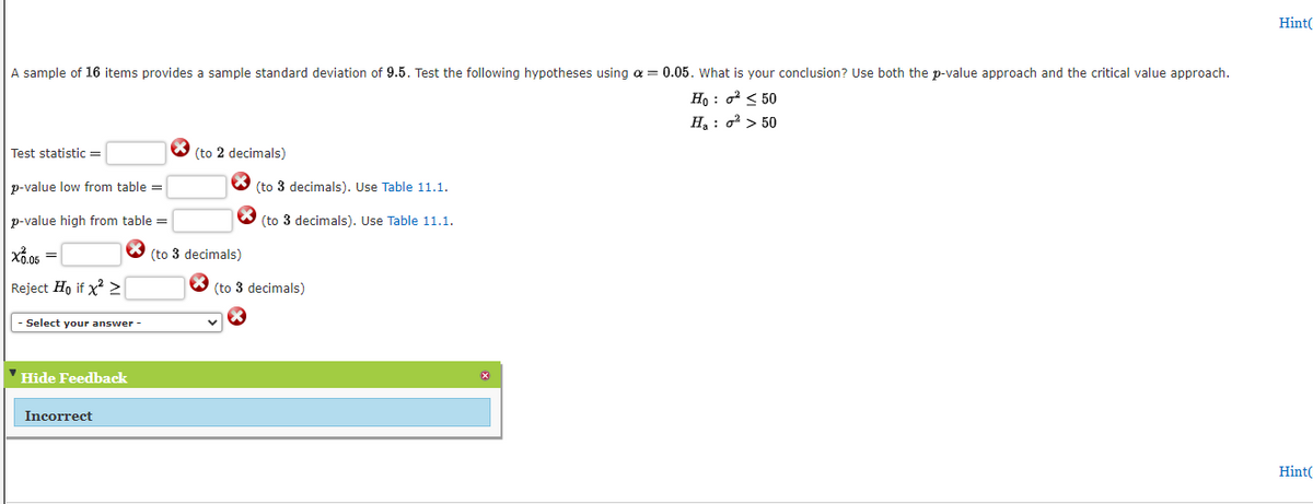
A sample of 16 items provides a sample standard deviation of 9.5. Test the following hypotheses using a = 0.05. What is your conclusion? Use both the p-value approach and the critical value approach. Ho: ² ≤ 50 ² > 50 H₂ : est statistic = -value low from table = D-value high from table= <.05=[ Reject Ho if x² 2 - Select your answer Hide Feedback Incorrect (to 2 decimals) (to 3 decimals) (to 3 decimals). Use Table 11.1. (to 3 decimals). Use Table 11.1. (to 3 decimals) x Hint( Hint(

On average, Americans have lived in 4 places by the time they are 18 years old. Is this average more for college students? The 52 randomly selected college students who answered the survey question had lived in an average of 4.18 places by the time they were 18 years old. The standard deviation for the survey group was 0.5. What can be concluded at the  αα = 0.05 level of significance?

I. A study reports that teenagers spend 27 hours a week online (www.telegraph.co.uk). A researcher wanted to check if this claim is true. A random sample of 200 teenagers taken showed that they spend an average of 25.7 hours per week online with a standard deviation of 8.2 hours. Perform a hypothesis test with the alternate hypothesis that teenagers spend less than 27 hours per week online. Use c = 0.05. Perform all of the steps outline in your notes and write a complete conclusion in words. Assume the distribution of hours spent online is normally distributed.

You wish to test the following claim (HaHa) at a significance level of α=0.001α=0.001.      Ho:μ=53.4      Ha:μ<53.4You believe the population is normally distributed, but you do not know the standard deviation. You obtain the following sample of data: What is the test statistic for this sample? (Report answer accurate to three decimal places.)test statistic = What is the p-value for this sample? (Report answer accurate to four decimal places.)p-value =   45.6 39.8 42.3 45.4 33.4 46.6

Arandom sample of 15 observations taken from a population that is normally distributed produced a sample mean of 42.4 and a standard deviation of 8. Find the range for the p-value and the critical and observed values of t for each of the following tests of hypotheses using, a= 0.01 Use the distribution table to find a range for the pvalue. Round your answers for the values of decimal places. H0: mean =46 versus H1: mean<46. = <p-value <p-value t critical=t observed= b. H0: mean=46 versus H1: mean≠46 = < p-value <   t critical left=t critical right=t observed=

Many people believe that the average number of Facebook friends is 150. The population standard deviation is 37.6. A random sample of 46 high school students in a particular county revealed that the average number of Facebook friends was 159. At =α0.01, is there sufficient evidence to conclude that the mean number of friends is greater than 150? A. State the hypotheses and identify the claim with the correct hypothesis. :H0 ▼claim or not claim :H1 ▼claim or not claimThis hypotheses test is a ▼one-tailed or two-tailed test B. Find the critical value(s) (c)Compute the test value. z= (d)Make the decision. reject or accept (e)Summarize the results. is there enough evidence to support the claim

A large milling machine produces steel rods to certain specifications. The machine is considered to be running normally if the standard deviation of the diameter of the rods is at most 0.15 millimeters. The line supervisor needs to test the machine is for normal functionality. The quality inspector takes a sample of 25 rods and finds that the sample standard deviation is 0.19. What are the null and alternative hypotheses for the test?   A. H0 : σ = 0.0225 and H1 : σ ≠ 0.0225   B. H0 : σ ≥ 0.15 and H1 : σ < 0.15     C. H0 : σ2 > 0.15 and H1 : σ2 ≤ 0.15     D. H0 : σ2 ≤ 0.0225 and H1 : σ2 > 0.0225

The average scores in a pre-final examination scored by under graduate students in the previous year was 63. A tutor, after conducting the weekly tests, wishes to check whether that average has increased this year. For a sample of 70 students, the mean score was 68 with a standard deviation of 15.State the null and the alternative hypotheses. Group of answer choices H0: μ = 63 vs. Ha: μ ≥ 63 H0: μ = 63 vs. Ha: μ ≠ 63 H0: μ = 63 vs. Ha: μ ≤ 63 H0: μ = 63 vs. Ha: μ > 63 H0: μ = 63 vs. Ha: μ < 63

A taxi company claims that its drivers have an average of at least 12.4 years' experience. In a study of 15 taxi drivers, the average experience was 11.2 years. The standard deviation was 2. At a = 0.10, is the number of years' experience of the taxi drivers really less than the taxi company claimed. State the hypotheses and identify the claim.Identify the statistical test to be used. a. Find for the critical value(s). b. Sketch a curve with the rejection and non-rejection region. Computer for the test value. c. Make the decision. Interpret the results.

Two samples are taken with the following sample means, standard deviations, and sample sizes. We have no reason to assume the variance are equal. T1 = 20 81 = 3 n₁ = 50 F₂ = 27 82 = 2 n₂ = 65 Estimate the difference in population means using a 88% confidence level in interval notation. Round answers to 2 decimal places. -7.770 -6.23 X