
MATLAB: An Introduction with Applications
6th Edition
ISBN: 9781119256830
Author: Amos Gilat
Publisher: John Wiley & Sons Inc
expand_more
expand_more
format_list_bulleted
Related questions
Question
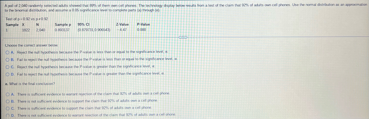

Transcribed Image Text:A poll of 2,040 randomly selected adults showed that 89% of them own cell phones. The technology display below results from a test of the claim that 92% of adults own cell phones. Use the normal distribution as an approximation
to the binomial distribution, and assume a 0.05 significance level to complete parts (a) through (e).
Test of p=0.92 vs p *0.92
Sample X
95% CI
N
2,040
Sample p
0.893137
Z-Value
P.Value
0.000
1
1822
(0.879731,0.906543) -4.47
Choose the correct answer below.
O A. Reject the null hypothesis because the P-value is less than or equal to the significance level, a.
OB. Fail to reject the null hypothesis because the P-value is less than or equal to the significance level, a.
OC. Reject the null hypothesis because the P-value is greater than the significance level, a.
OD. Fail to reject the null hypothesis because the P-value is greater than the significance level, a
e. What is the final conclusion?
OA. There is sufficient evidence to warrant rejection of the claim that 92% of adults own a cell phone.
OB. There is not sufficient evidence to support the claim that 92% of adults own a cell phone.
OC. There is sufficient evidence to support the claim that 92% of adults own a cell phone.
D. There is not sufficient evidence to warrant reiection of the claim that 92% of adults own a cell phone.
Expert Solution
This question has been solved!
Explore an expertly crafted, step-by-step solution for a thorough understanding of key concepts.

Step by stepSolved in 2 steps with 2 images

Knowledge Booster

Similar questions
- On a particular production line, the likelihood that a light bulb is defective is 5%. Ten light bulbs are randomly selected. What are the mean and variance of the number of defective bulbs?arrow_forwardWhich is not one of the major assumptions typically associated with parametric tests of significance? A. Random Selection B. Homogeneity of Variance C. Absence of restricted rangesarrow_forwardWhich samples show unequal variances? Use a = .10 in all tests. Show the critical values and degrees of freedom clearly and illustrate the decision rule. s1 = 10.2, n1 = 22, s2 = 6.4, n2 = 16, two-tailed test s1 = .89, n1 = 25, s2 = .67, n2 = 18, right tailed test s1 = 124, n1 = 12, s2 = 260, n2 = 10, left-tailed testarrow_forward
- Use the Excel printout to answer the following questions. t-Test: Two-Sample Assuming Equal Variances E Variable 1 Variable 2 Mean 28.671 28.215 Variance 5.061 2.225 Observations 8 7 Pooled Variance 3.752 Hypothesized Mean Difference df 13 t Stat 0.455 P(T <= t) one-tail 0.328 t Critical one-tail 1.771 P(T <= t) two-tail 0.657 t Critical two-tail 2.160 In testing for a difference between the two population means, would you conclude that the assumption of a common variance is reasonable? O Yes, the ratio of the the larger variance to the smaller variance is less than three. O Yes, the ratio of the larger variance to the smaller variance is more than three. O No, the ratio of the larger variance to the smaller variance is less than three. O No, the ratio of the larger variance to the smaller variance is more than three. O It is not possible to check that assumption with the given information. What is the observed value of the test statistic? t = What are the degrees of freedom for the…arrow_forwardDo cars really get better mileage per gallon on the highway? The table shows results from a study of the MPG (miles per gallon) of cars both in the city and on the highway. Assume that the two samples are randomly selected, independent, the population standard deviations are not know and not considered equal. At the 0.1 significance level, test the claim that the mpg on the highway is better than in the city. MPG on the Highway 35.6 34.3 32.2 33.9 31.1 27.1 33.3 33.4 29.3 33.5 31.4 33.2 33.5 30.8 33.8 MPG in the City 26.4 25.3 18.6 25.6 24.7 24.6 25.1 22.4 29.3 23.7 23.4 22 24 23.6 25.5 What are the correct hypotheses? (Select the correct symbols and use decimal values not percentages.)H0: Select an answer p x̄₁ p₁ σ₁² μ₁ μ₂ μ μ(Highway) x̄₂ p̂₁ s₁² p₂ ? ≤ ≠ < ≥ = > Select an answer p₁ p₂ p̂₁ μ(City) μ μ₁ μ₂ x̄₁ x̄₂ s₁² σ₁² p H1: Select an answer p₂ μ(Highway) p̂₂ σ₂² x̄₁ x̄₂ s₂² μ₁ μ₂ μ p₁ p ? < ≠ = ≥ ≤ > Select an answer p₂ p₁ μ₁ σ₁²…arrow_forwardA study was done using a treatment group and a placebo group. The results are shown in the table. Assume that the two samples are independent simple random samples selected from normally distributed populations, and do not assume that the population standard deviations are equal. Complete parts (a) and (b) below. Use a 0.10 significance level for both parts. a. Test the claim that the two samples are from populations with the same mean. What are the null and alternative hypotheses? OA. Ho: H₁ H₂ H₁: Hq ZH₂ OC. Ho: H₁ H₂ H₁: Hy > H₂ The test statistic, t, is. (Round to two decimal places as needed.) (Round to three decimal places as needed.) The P-value is State the conclusion for the test. C... OB. Ho: H₁ H₂ H₁: Hy #H₂ OD. Ho: Hg #U2 H₁: Hyarrow_forward
- A study was done using a treatment group and a placebo group. The results are shown in the table. Assume that the two samples are independent simple random samples selected from normally distributed populations, and do not assume that the population standard deviations are equal. Complete parts (a) and (b) below. Use a 0.01 significance level for both parts. a. Test the claim that the two samples are from populations with the same mean. What are the null and alternative hypotheses? OA. Ho H1 H2 H₁: H1 H2 The test statistic, t, is -1.55. (Round to two decimal places as needed.) The P-value is (Round to three decimal places as needed.) OB. Ho: H1 H2 H₁₁₂ D. Ho: H1 H2 H₁: H1 H2 Treatment Placebo μ H₁ H2 n 25 40 X 2.38 2.65 S 0.53 0.87arrow_forwardA study was done using a treatment group and a placebo group. The results are shown in the table. Assume that the two samples are independent simple random samples selected from normally distributed populations, and do not assume that the population standard deviations are equal. Complete parts (a) and (b) below. Use a 0.01 significance level for both parts. a. Test the claim that the two samples are from populations with the same mean. What are the null and alternative hypotheses? OA. Ho: H₁ H₂ H₁: H₁ H₂ OC. Ho: H₁ H¹/₂ H₁: H₁arrow_forwardGiven below are the analysis of variance results from a stat software display comparing sample data for the meanmileage for 4 different types of cars. Assume that you want to use a 0.05 significance level in testing the null hypothesisthat the different samples come from cars with the same mileage. What can you conclude about the equality of the population means?Source DF SS MS F pFactor 3 13.500 4.500 5.17 0.011Error 16 13.925 0.870Total 19 27.425 12)What is the null and alternative hypothesis for this scenari?Based on this One Way Anova software analysis, would you reject of fail to reject the nul hypothesis?What does this result mean in context?arrow_forward
- Please help me answer this question in full!arrow_forwardPerform an analysis of variance (ANOVA) to determine if the differences in the percentage butterfat of the different breeds of cows is statistically significant. Guernsey Jersey Holstein 4.51 4.59 3.43 5.26 6.67 3.68 5.81 5.39 3.72 5.14 4.38 3.76 4.55 4.99 4.43 4.86 5.49 3.84 4.69 5.43 3.54 4.12 5.02 4.18 5.44 5.16 3.4 4.69 5.15 3.77 5.24 5.76 4.03 4.62 5.34 3.63 4.61 5.11 3.37 5.02 4.75 3.54 4.67 5.07 3.64 4.59 4.42 3.98 4.92 6.13 5.58 4.6 5.6 5.83 1. Compute the treatment sum of squares (SSTr) and the error sum of squares (SSE) and use them to complete the following ANOVA table. (Round your answers to 4 decimal places). Source S.S. df M.S. F Treatment Error Total 2. Compute the p-value. (Round your answer to 4 decimal places.)p-value =arrow_forward
arrow_back_ios
arrow_forward_ios
Recommended textbooks for you
- MATLAB: An Introduction with ApplicationsStatisticsISBN:9781119256830Author:Amos GilatPublisher:John Wiley & Sons Inc
 Probability and Statistics for Engineering and th...StatisticsISBN:9781305251809Author:Jay L. DevorePublisher:Cengage Learning
 Statistics for The Behavioral Sciences (MindTap C...StatisticsISBN:9781305504912Author:Frederick J Gravetter, Larry B. WallnauPublisher:Cengage Learning
  Elementary Statistics: Picturing the World (7th E...StatisticsISBN:9780134683416Author:Ron Larson, Betsy FarberPublisher:PEARSON
 The Basic Practice of StatisticsStatisticsISBN:9781319042578Author:David S. Moore, William I. Notz, Michael A. FlignerPublisher:W. H. Freeman
 Introduction to the Practice of StatisticsStatisticsISBN:9781319013387Author:David S. Moore, George P. McCabe, Bruce A. CraigPublisher:W. H. Freeman
MATLAB: An Introduction with Applications
Statistics
ISBN:9781119256830
Author:Amos Gilat
Publisher:John Wiley & Sons Inc
Probability and Statistics for Engineering and th...
Statistics
ISBN:9781305251809
Author:Jay L. Devore
Publisher:Cengage Learning
Statistics for The Behavioral Sciences (MindTap C...
Statistics
ISBN:9781305504912
Author:Frederick J Gravetter, Larry B. Wallnau
Publisher:Cengage Learning
Elementary Statistics: Picturing the World (7th E...
Statistics
ISBN:9780134683416
Author:Ron Larson, Betsy Farber
Publisher:PEARSON
The Basic Practice of Statistics
Statistics
ISBN:9781319042578
Author:David S. Moore, William I. Notz, Michael A. Fligner
Publisher:W. H. Freeman
Introduction to the Practice of Statistics
Statistics
ISBN:9781319013387
Author:David S. Moore, George P. McCabe, Bruce A. Craig
Publisher:W. H. Freeman