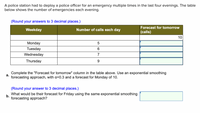
A police station had to deploy a police officer for an emergency multiple times in the last four evenings. The table below shows the number of emergencies each evening. (Round your answers to 3 decimal places.) Forecast for tomorrow Weekday Number of calls each day |(calls) 10 Monday Tuesday 6. Wednesday 7 Thursday 9. Complete the "Forecast for tomorrow" column in the table above. Use an exponential smoothing a. forecasting approach, with a=0.3 and a forecast for Monday of 10. (Round your answer to 3 decimal places.) What would be their forecast for Friday using the same exponential smoothing b. forecasting approach?

Data collected on the yearly registrations for a Six Sigma seminar at the Quality College are shown in the following table: Year Year Forecast (000) 1 2 4.00 7.00 1 5.00 3 5.00 Registrations (000) a) Calculate the forecasted registrations for years 2 through 12 using exponential smoothing, with a smoothing constant (a) of 0.40 and a starting forecast of 5.00 for year 1 (round your responses to one decimal place): 2 3 4.6 5.56 4 4.00 4 5.34 11 9 10 7 8 6 5 9.00 9.00 6.00 10.00 13.00 14.00 12.00 5 4.80 6 7 6.48 7.49 8 6.89 9 8.14 10 10.08 11 11.64 12 11.79 b) Mean absolute deviation based on the forecast developed using the exponential smoothing method (with a smoothing constant (a) = 0.40 and a starting forecast of F₁ = 5.00) is response to one decimal place). registrations (round your

A police station had to deploy a police officer for an emergency multiple times in the last four evenings. The t below shows the number of emergencies each evening. Weekday Number of calls each day Monday 10 Tuesday 2 Wednesday 12 Thursday 12 (Round your answer to 1 decimal place.) What would be their forecast for the emergencies on Friday using a two-day moving average approach? Forecast for Friday calls

One forecasting model was used to forecast demand for a product. The forecasts and the demand are shown in the table below. Use two decimals in your answer. Actual Forecast 1 40 41 2 35 38 3 38 35 4 33 30 The Mean Absolute Deviation (MAD) is O 0.5 2.5 O 1.48 7.01

A security company had to deploy guards for emergencies multiple times in the last four evenings. The numbers of emergencies for Monday, Tuesday, Wednesday, and Thursday were 7, 4, 8, and 11, respectively. What would be the security company's forecast for the number of emergencies on Friday using an exponential smoothing forecasting approach? (Use \alpha= 0.2 and a forecast for Monday of 10 emergencies)

Here are the actual tabulated demands for an item for a nine-month period (January through September). Your supervisor wants to test two forecasting methods to see which method was better over this period.   MONTH ACTUAL January 120 February 145 March 146 April 171 May 154 June 182 July 138 August 135 September 146     a. Forecast April through September using a three-month moving average. b. Use simple exponential smoothing with an alpha of  0.20 to estimate April through September, using the average of January through March as the initial forecast for April.  c-1. Calculate MAD for Three-month moving average and Exponential smoothing. c-2. Use MAD to decide which method produced the better forecast over the six-month period.

Give typed explanation Part 2: Using exponential smoothing, the forecasted demand for period 5 using the smoothing constant determined in image= ?

If month one has 240,000 demands, month two 250,080 demands, month three 325,00 demands, month four 370,000 demands, month five 420,000 demands and month six 509,00 demands. Use a forecast for the first month of 240,000, an initial trend forecast of 50,000, and smoothing parameters of 0.35 for both demand smoothing and trend smoothing. Compute the forecasts and trends using double exponential smoothing

Amazon finds that sales in July are much greater relative to other months because of the Amazon Prime days in that month. Assuming that an exponential smoothing model is used for forecasting sales, what should the company best do to make the forecast for the next month (Aug) more reflective of reality? Please pick from the provided options.    F t+1 = αDt + (1-α) Ft     increase value of alpha     decrease value of alpha     stay with the same alpha     decrease the expected forecast for the current month (Ft)     On hearing our forecast, our clients probe - how sure are we about the forecast?  Which measure of errror (among those stated below) should we best use to respond?     a. Root MSE (RMSE)     b. Mean absolute percentage error (MAPE)     c. Mean forecast error (Avg. error)     d. Cumulative forecast error (CFE)

d) Using exponential smoothing with α ​= 0.40 and the forecast for year 1 being 3,000​, the forecast for year 6​ = ? miles ​(round your response to the nearest whole​ number).