
MATLAB: An Introduction with Applications
6th Edition
ISBN: 9781119256830
Author: Amos Gilat
Publisher: John Wiley & Sons Inc
expand_more
expand_more
format_list_bulleted
Related questions
Topic Video
Question
Help please!!
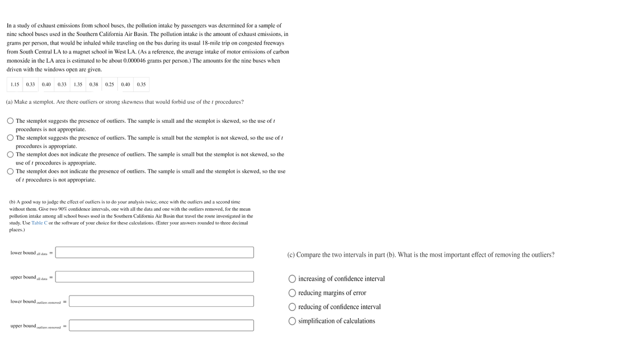

Transcribed Image Text:In a study of exhaust emissions from school buses, the pollution intake by passengers was determined for a sample of
nine school buses used in the Southern California Air Basin. The pollution intake is the amount of exhaust emissions, in
grams per person, that would be inhaled while traveling on the bus during its usual 18-mile trip on congested freeways
from South Central LA to a magnet school in West LA. (As a reference, the average intake of motor emissions of carbon
monoxide in the LA area is estimated to be about 0.000046 grams per person.) The amounts for the nine buses when
driven with the windows open are given.
1.15
0.33
0.40
0.33
1.35
0.38
0.25
0.40
0.35
(a) Make a stemplot. Are there outliers or strong skewness that would forbid use of the t procedures?
The stemplot suggests the presence of outliers. The sample is small and the stemplot is skewed, so the use of t
procedures is not appropriate.
The stemplot suggests the presence of outliers. The sample is small but the stemplot is not skewed, so the use of t
procedures is appropriate.
The stemplot does not indicate the presence of outliers. The sample is small but the stemplot is not skewed, so the
use of t procedures is appropriate.
The stemplot does not indicate the presence of outliers. The sample is small and the stemplot is skewed, so the use
of t procedures is not appropriate.
(b) A good way to judge the effect of outliers is to do your analysis twice, once with the outliers and a second time
without them. Give two 90% confidence intervals, one with all the data and one with the outliers removed, for the mean
pollution intake among all school buses used in the Southern California Air Basin that travel the route investigated in the
study. Use Table C or the software of your choice for these calculations. (Enter your answers rounded to three decimal
places.)
lower bound all data
(c) Compare the two intervals in part (b). What is the most important effect of removing the outliers?
upper bound
O increasing of confidence interval
%3D
all data
reducing margins of error
lower bound outliers removed =
reducing of confidence interval
O simplification of calculations
upper bound outliers removed

Transcribed Image Text:TABLES
699
Table entry for C is the critical value
t* required for confidence level C.
To approximate one- and two-sided
P-values, compare the value of the t
Tail area
statistic with the critical values of t*
Area C
that match the P-values given at the
bottom of the table.
t*
TABLE C t distribution critical values
Confidence level C
Degrees of
freedom
50%
60%
70%
80%
90%
95%
96%
98%
99%
99.5%
99.8%
99.9%
1
1.000
1.376
1.963
3.078
6.314
12.71
15.89
31.82
63.66
127.3
318.3
636.6
0.816
1.061
1.386
1.886
2.920
4.303
4.849
6.965
9.925
14.09
22.33
31.60
1.250
7.453
5.598
3
0.765
0.978
1.638
2.353
3.182
3.482
4.541
5.841
10.21
12.92
4
0.741
0.941
1.190
1.533
2.132
2.776
2.999
3.747
4.604
7.173
8.610
0.727
0.920
1.156
1.476
2.015
2.571
2.757
3.365
4.032
4.773
5.893
6.869
6.
0.718
0.906
1.134
1.440
1.943
2.447
2.612
3.143
3.707
5.208
4.317
4.029
5.959
7
0.711
0.896
1.119
1.415
1.895
2.365
2.517
2.998
3.499
4.785
5.408
8
0.706
0.889
1.108
1.397
1.860
2.306
2.449
2.896
3.355
3.833
4.501
5.041
9.
0.703
0.883
1.100
1.383
1.833
2.262
2.398
2.821
3.250
3.690
4.297
4.781
10
0.700
0.879
1.093
1.372
1.812
2.228
2.359
2.764
3.169
3.581
4.144
4.587
11
0.697
0.876
1.088
1.363
1.796
2.201
2.328
2.718
3.106
3.497
4.025
4.437
12
0.695
0.873
1.083
1.356
1.782
2.179
2.303
2.681
3.055
3.428
3.930
4.318
13
0.694
0.870
1.079
1.350
1.771
2.160
2.282
2.650
3.012
3.372
3.852
4.221
14
0.692
0.868
1.076
1.345
1.761
2.145
2.264
2.624
2.977
3.326
3.787
4.140
15
0.691
0.866
1.074
1.341
1.753
2.131
2.249
2.602
2.947
3.286
3.733
4.073
16
0.690
0.865
1.071
1.337
1.746
2.120
2.235
2.583
2.921
3.252
3.686
4.015
17
0.689
0.863
1.069
1.333
1.740
2.110
2.224
2.567
2.898
3.222
3.646
3.965
18
0.688
0.862
1.067
1.330
1.734
2.101
2.214
2.552
2.878
3.197
3.611
3.922
1.066
1.064
1.729
1.725
19
0.688
0.861
1.328
2.093
2.205
2.539
2.861
3.174
3.579
3.883
20
0.687
0.860
1.325
2.086
2.197
2.528
2.845
3.153
3.552
3.850
1.063
1.323
3.135
3.527
3.505
21
0.686
0.859
1.721
2.080
2.189
2.518
2.831
3.819
0.858
0.858
22
0.686
1.061
1.321
1.717
2.074
2.183
2.508
2.819
3.119
3.792
23
0.685
1.060
1.319
3.485
1.714
1.711
2.069
2.177
2.500
2.807
3.104
3.768
24
0.685
0.857
1.059
1.318
2.064
2.172
2.492
2.797
3.091
3.467
3.745
25
0.684
0.856
1.058
1.316
1.708
2.060
2.167
2.485
2.787
3.078
3.450
3.725
26
0.684
0.856
1.058
1.315
1.706
2.056
2.162
2.479
2.779
3.067
3.435
3.707
27
0.684
0.855
1.057
1.314
1.703
2.052
2.158
2.473
2.771
3.057
3.421
3.690
28
0.683
0.855
1.056
1.313
1.701
2.048
2.154
2.467
2.763
3.047
3.408
3.674
29
0.683
0.854
1.055
1.311
1.699
2.045
2.150
2.462
2.756
3.038
3.396
3.659
30
0.683
0.854
1.055
1.310
1.697
2.042
2.147
2.457
2.750
3.030
3.385
3.646
40
0.681
0.851
1.050
1.303
1.684
2.021
2.123
2.423
2.704
2.971
3.307
3.551
0.679
0.679
50
0.849
1.047
1.299
1.676
2.009
2.109
2.403
2.678
2.937
3.261
3.496
60
0.848
1.045
1.296
1.671
2.000
2.099
2.390
2.660
2.915
3.232
3.460
80
0.678
0.846
1.043
1.292
1.664
1.990
2.088
2.374
2.639
2.887
3.195
3.416
100
0.677
0.845
1.042
1.290
1.660
1.984
2.081
2.364
2.626
2.871
3.174
3.390
1000
0.675
0.842
1.037
1.282
1.646
1.962
2.056
2.330
2.581
2.813
3.098
3.300
0.674
0.841
1.036
1.282
1.645
1.960
2.054
2.326
2.576
2.807
3.091
3.291
One-sided P
.25
.20
.15
.10
.05
.025
.02
.01
.005
.0025
.001
.0005
Two-sided P
.50
.40
.30
.20
.10
.05
.04
.02
.01
.005
.002
.001
Expert Solution
This question has been solved!
Explore an expertly crafted, step-by-step solution for a thorough understanding of key concepts.

This is a popular solution

Trending nowThis is a popular solution!

Step by stepSolved in 2 steps with 4 images

Knowledge Booster


Learn more about
Need a deep-dive on the concept behind this application? Look no further. Learn more about this topic, statistics and related others by exploring similar questions and additional content below.Similar questions
arrow_back_ios
arrow_forward_ios
Recommended textbooks for you
- MATLAB: An Introduction with ApplicationsStatisticsISBN:9781119256830Author:Amos GilatPublisher:John Wiley & Sons Inc
 Probability and Statistics for Engineering and th...StatisticsISBN:9781305251809Author:Jay L. DevorePublisher:Cengage Learning
 Statistics for The Behavioral Sciences (MindTap C...StatisticsISBN:9781305504912Author:Frederick J Gravetter, Larry B. WallnauPublisher:Cengage Learning
  Elementary Statistics: Picturing the World (7th E...StatisticsISBN:9780134683416Author:Ron Larson, Betsy FarberPublisher:PEARSON
 The Basic Practice of StatisticsStatisticsISBN:9781319042578Author:David S. Moore, William I. Notz, Michael A. FlignerPublisher:W. H. Freeman
 Introduction to the Practice of StatisticsStatisticsISBN:9781319013387Author:David S. Moore, George P. McCabe, Bruce A. CraigPublisher:W. H. Freeman
MATLAB: An Introduction with Applications
Statistics
ISBN:9781119256830
Author:Amos Gilat
Publisher:John Wiley & Sons Inc
Probability and Statistics for Engineering and th...
Statistics
ISBN:9781305251809
Author:Jay L. Devore
Publisher:Cengage Learning
Statistics for The Behavioral Sciences (MindTap C...
Statistics
ISBN:9781305504912
Author:Frederick J Gravetter, Larry B. Wallnau
Publisher:Cengage Learning
Elementary Statistics: Picturing the World (7th E...
Statistics
ISBN:9780134683416
Author:Ron Larson, Betsy Farber
Publisher:PEARSON
The Basic Practice of Statistics
Statistics
ISBN:9781319042578
Author:David S. Moore, William I. Notz, Michael A. Fligner
Publisher:W. H. Freeman
Introduction to the Practice of Statistics
Statistics
ISBN:9781319013387
Author:David S. Moore, George P. McCabe, Bruce A. Craig
Publisher:W. H. Freeman