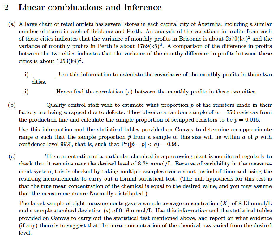
A large chain of retail outlets has several stores in each capital city of Australia, including a similar number of stores in each of Brisbane and Perth. An analysis of the variations in profits from each of these cities indicates that the variance of monthly profits in Brisbane is about 2570(k$)2 and the variance of monthly profits in Perth is about 1789(k$)2. A comparison of the difference in profits between the two cities indicates that the variance of the monthy difference in profits between these cities is about 1253(k$)². i) Use this information to calculate the covariance of the monthly profits in these two Hence find the correlation (p) between the monthly profits in these two cities. ii) cities.

Noise pollution is measured in decibels. In California any motorcycle made after 1980 may not be any louder than 80 decibels.  Harley Davidson claims their mean decibel rating on bikes is 70 with a variance of 10.  The variance of the noise is questioned.  Just because Harley has a mean that is less than 80, they could still be producing louder than acceptable bikes.  The federal EPA conducts a sample of 30 bikes and determines the variance to be 20 decibels.  Is there enough evidence to question Harley’s claim of 10 decibels?

Suppose the variance of X is 14. What is the variance of .47X?

Actuaries use various parameters when evaluating the cost of a life insurance policy. The variance of the life spans of a population is one of the parameters used for the evaluation. Each year, the actuaries at a particular insurance company randomly sample 30 people who died during the year (with the samples chosen independently from year to year) to see whether the variance of life spans has changed. The life span data from this year and from last year are summarized below. Current Last Year Year x1 = 75.8 | x,= 76.2 si= 47.61 s3= = 92.16 (The first row gives the sample means and the second row gives the sample variances.) Assume that life spans are approximately normally distributed for each of the populations of people who died this year and people who died last year. Can we conclude, at the 0.05 significance level, that the variance of the life span for the current year, of, differs from the variance of the life span for last year, o,? Perform a two-tailed test. Then complete the…