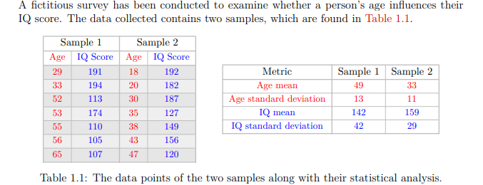
A fictitious survey has been conducted to examine whether a person's age influences their IQ score. The data collected contains two samples, which are found in Table 1.1. Sample 1 Age IQ Score 29 33 52 53 55 56 65 191 194 113 174 110 105 107 Sample 2 Age IQ Score 18 20 30 35 38 43 47 192 182 187 127 149 156 120 Metric Age mean Age standard deviation IQ mean IQ standard deviation Sample 1 Sample 2 49 33 13 11 142 42 159 29 Table 1.1: The data points of the two samples along with their statistical analysis.

Identify the range, variance and standard deviation. show complete solutions

Listed below are systolic blood pressure measurements (mm Hg) taken from the right and left arms of the same woman. ASsume that the paired sample data is a simple random sample and that the differences have a distribution that is approximately normal. Use a 0.05 significance level to test for a difference between the measurements from the two arms. What can be concluded? 146 144 123 137 139 Right arm Left arm 185 174 187 151 137 In this example, µa is the mean value of the differences d for the population of all pairs of data, where each individual differenced is defined as the measurement from the right arm minus the measurement from the left arm. What are the null and alternative hypotheses for the hypothesis test? O A. Ho: Hd #0 O B. Ho: Ha 0 Hd. 0 Prl : H Identify the test statistic. t= (Round to two decimal places as needed.) Identify the P-value. P-value = (Round to three decimal places as needed.) What is the conclusion based on the hypothesis test? Since the P-value is than…

Below is a random sample of measured verbal IQ (IQV) scores from 20 children.   61 82 70 72 72 95 89 57 116 95 82 116 99 74 100 72 126 80 86 94   Include appropriate titles and labels as you complete the following:  Construct a stem and leaf plot for the data.  Find the mean, median, & mode of the data. Find the range, variance, and standard deviation of the data.