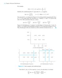
Figure attached below.1. A bin of 5 transistors is known to contain 2 that are defective. The transistors are to be tested, one at atime, until the defective ones are identified. Denote by X the number of tests made until the first defectis identified and by Y the number of additional tests until the second defect is identified.(a) Find g(x|y) and draw a figure like Figure 4.3-1(b), depicting the conditional pmfs fory = 1,2,3,and 4.(b) Find h(y|x) and draw a figure like Figure 4.3-1(c), depicting the conditional pmfs forx = 1,2,3,and 4.(c) Find E [X|Y = 2] and Var (X|Y = 2) 146 Chapter 4 Bivariate DistributionsFor example,41P(X = 2|Y = 2) = g(2|2) =123Similarly, the conditional pmf of Y, given that X= x, is equal tox+ yh(y|x) =y = 1, 2, when x =1, 2, or 3.2x + 3The joint pmf f(x, y) is depicted in Figure 4.3-1(a) along with the marginal pmfs. Now,if y = 2, we would expect the outcomes of x-namely, 1, 2, and 3–to occur in theratio 3:4:5. This is precisely what g(x|y) does:1+22+23+2g(1|2)g(2|2) =12g(3|2) :1212Figure 4.3-1(b) displays g(x|1) and g(x|2), while Figure 4.3-1(c) gives h(y|1), h(y|2),and h(y|3). Compare the probabilities in Figure 4.3-1(c) with those in Figure 4.3-1(a).They should agree with your intuition as well as with the formula for h(y|x).fy(y)y12/21 2• 3/21• 4/21• 5/219/21 1• 2/21• 3/21• 4/211235/217/219/21fx(x)(a) Joint and marginal pmfsyyh(y|1)h(y|2)h(y|3)• 3/12• 4/12• 5/12 g(x|2)2• 3/5• 4/7• 5/91• 2/9• 3/9• 4/9g(x|1)1• 2/5• 3/7• 4/9123123(b) Conditional pmfs of X, given y(c) Conditional pmfs of Y, given xFigure 4.3-1 Joint, marginal, and conditional pmfsNote that 0

Conditional probability Given discrete random variables, X and Y with joint probability mass…

Answered: A bin of 5 transistors is known to…

Calculus For The Life Sciences

2nd Edition

ISBN:9780321964038

Author:GREENWELL, Raymond N., RITCHEY, Nathan P., Lial, Margaret L.

Publisher:GREENWELL, Raymond N., RITCHEY, Nathan P., Lial, Margaret L.

Chapter2: Exponential, Logarithmic, And Trigonometric Functions

Section2.CR: Chapter 2 Review

Problem 111CR: Respiratory Rate Researchers have found that the 95 th percentile the value at which 95% of the data...

See similar textbooks

Related questions

Question

Figure attached below.

1. A bin of 5 transistors is known to contain 2 that are defective. The transistors are to be tested, one at a
time, until the defective ones are identified. Denote by X the number of tests made until the first defect
is identified and by Y the number of additional tests until the second defect is identified.
(a) Find g(x|y) and draw a figure like Figure 4.3-1(b), depicting the conditional pmfs for
y = 1,2,3,and 4.
(b) Find h(y|x) and draw a figure like Figure 4.3-1(c), depicting the conditional pmfs for
x = 1,2,3,and 4.
(c) Find E [X|Y = 2] and Var (X|Y = 2)