
MATLAB: An Introduction with Applications
6th Edition
ISBN: 9781119256830
Author: Amos Gilat
Publisher: John Wiley & Sons Inc
expand_more
expand_more
format_list_bulleted
Related questions
Concept explainers
Question
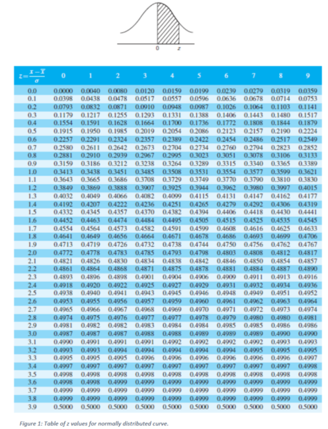
A batch of 3000 inverters from the production line has a mean output voltage of 337.8 V and the Standard deviation of the output voltage is 3.105. If the voltages of the produced inverters are assumed to be
- The number of inverters with output voltages greater than 336.9 V.
- The number of inverters with output voltages less than 337.1 V,
- The number of inverters with output voltages between 336.2 V and 339.8 V.
For this problem you should use the table of z-values shown in Figure below.

Transcribed Image Text:I-
01 2 3 4 s
6 7 8
0.0
0.1
0.0000 0.0040 0.0080 0.0120 0.0159 0.0199 0.0239 0.0279 0.0319 0.0359
0.0398 0.0438 0.0478 0.0517 0.0557 0.0596 0.0636 0.0678 0.0714 0.0753
0.2
0.3
0.0793 0.0832 0.0871 0.0910
0.1179 0.1217 0.1255 0.1293 0.1331
0.1554 0.1591 0.1628 0.1664 0.1700 0.1736 0.1772 0.1808
0.1915 0.1950 0.1985 0.2019 0.2054 0.2086 0.2123 0.2157 0.2190 0.2224
0.0948 0.0987 0.1026 0.1064 0.1103 0.1141
0.1388 0.1406 0.1443 0.1480 0.1517
0.1844 0.1879
0.4
0.5
0.6
0.2257 0.2291
0.2324 0.2357 0.2389 0.2422 0.2454 0.2486 0.2517 0.2549
0.7
0.2580 0.2611 0.2642 0.2673 0.2704 0.2734 0.2760 0.2794 0.2823 0.2852
0.2881
0.3159
0.2910 0.2939 0.2967
0.3186 0.3212 0.3238 0.3264
0.3438
0.2995
0.3023 0.3051
0.3289 0.331I5 0.3340
0.3078
0.3106 0.3133
0.3365
0.8
0.9
0.3389
1.0
0.3485
0.3708 0.3729 0.3749 0.3770 0.3790 0.3810
0.3907 0.3925 0.3944
0.3531
0.3413
0.3643 0.3665
0.3849
0.3451
0.3686
0.3508
0.3554 0.3577 0.3599 0.3621
1.1
0.3830
1.2
0.3869
0.3888
0.3962
0.3980
0.3997
0.4015
1.3
14
15
0.4032 0.4049 0.4066 0.4082 0.4099 0.4115
0.4192
0.4332 0.4345 0,4357 0.4370 0,4382 0.4394
0.4131 0,4147 0,4162 04177
0.4292
0.4306
0.4207 0.4222 0.4236 04251
0.4265
0.4279
0.4319
0.4406 0.4418 0.4430 04441
1.6
1.7
0.4452
0.4554 0.4564 0.4573 0.4582 0.4591
0.4641 0.4649 0,4656 0,4664 0.4671
0.4713
0.4474 0.4484
0.4495 0.4505 0.4515
0.4599
4525 0.4535
0.4625
0.4699
0.4545
0.4608
0.4616
0.4633
0.4706
1.8
0.4678
0.4686
0.4693
1.9
0.4719 0.4726 0.4732 0.4738 0.4744 0.4750 0.4756 0.4762 04767
0.4812 0.4817
0.4808
0.4850 0.4854
0.4884 0.4887
2.0
0.4772 0.4778 0.4783
0.4785 0.4793 0.4798
0.4803
2.1
2.2
0.4821
0.4861
0.4893
0.4826
0.4830 0,4834
0.4838
0.4842
0.4846
0.4857
0.4864
0.4868 0.4871
0.4875
0.4878
0.4881
0.4890
2.3
0.4896
0.4898 0.4901
0.4904
0.4906
0.4909
0.4911
0.4913
0.4916
2.4
2.5
0.4920
0.4922
0.4940 0.4941
0.4925
0.4943 0.4945 0.4946
0.4918
0.4927
0.4929
0.4932 0,4934
0.4948 0.4949 0.4951 0.4952
0.4931
0.4936
0.4938
0.4953
0.4955
0.4962
0.4970 0.4971 0.4972 0.4973
0.4979
2.6
0.4956 0.4957
0.4959
0.4960
0.4961
0.4963
0.4964
2.7
0.4965
0.4966
0.4967
0.4968
0.4969
0.4974
0.4975
0.4980
2.8
2.9
0.4974
0.4981
0.4978
0.4982 0.4982 0.4983 0.4984 0.4984 0.4985 0.4985 0.4986 0.4986
0.4976
0.4977
0.4977
0.4980
0.4981
3.0
0.4987
0.4987 0.4987 0.4988 0.4988 0.4989 0.4989 0.4989 0.4990 0.4990
3.1
0.4990
0.4991
0.4991
0.4991
0.4992 0.4992 0.4992 0.4992 0.4993
0.4993
3.2
3.3
0.4993
0.4993
0.4994
0.4995 0.4995 0.4996
0.4994
0,4994
0.4994
0.4994
0.4995
0.4996 0.4996 0.4997
0.4995
0.4995
0.4995
0.4996 0.4996 0.4996
3.4
0.4997
0.4997 0.4997 0.4997 0.4997 0.4997 0.4997
0.4997 0.4997
0.4998
3.5
3.6
3.7
0.4998
0.4998
0.4998 0.4998 0.4998 0.4998 0.4998
0.4998
0.4998 0.4998
0.4998
0.4998 0.4999 0.4999 0.4999 0.4999 0.4999 0.4999 0.4999
0.4999
0.4999
0.4999 0.4999 0.4999 0.4999
0.4999
0.4999
0.4999
0.4999
0.4999
3.8
0.4999
0.4999 0.4999 0.4999 0,4999 0.4999
0.4999
0.4999
0.4999
0,4999
3.9
0.5000 0.5000 0.5000 0.5000 0.5000 0.5000
0.5000
0.5000
0.5000
0.5000
Figure 1: Table of z values for normally distributed curve.
Expert Solution
This question has been solved!
Explore an expertly crafted, step-by-step solution for a thorough understanding of key concepts.

Step by stepSolved in 4 steps with 4 images

Knowledge Booster


Learn more about
Need a deep-dive on the concept behind this application? Look no further. Learn more about this topic, statistics and related others by exploring similar questions and additional content below.Similar questions
- At a hair salon, customers arrive at the rate of 3 customers per hour. The standard deviation of the time between two consecutive arrivals is estimated as 9 minutes. On average, it takes a customer 25 minutes to complete the service (regardless of which hairdresser provides the service). The coefficient of variation of the service time is estimated as 0.8. What is the standard deviation of the service time in minutes?arrow_forwardWeatherwise is a magazine published by the American Meteorological Society. One issue gives a rating system used to classify Nor'easter storms that frequently hit New England and can cause much damage near the ocean. A severe storm has an average peak wave height of ? = 16.4 feet for waves hitting the shore. Suppose that a Nor'easter is in progress at the severe storm class rating. Peak wave heights are usually measured from land (using binoculars) off fixed cement piers. Suppose that a reading of 35 waves showed an average wave height of x = 17.3 feet. Previous studies of severe storms indicate that ? = 3.5 feet. Does this information suggest that the storm is (perhaps temporarily) increasing above the severe rating? Use ? = 0.01. (a) What is the level of significance?State the null and alternate hypotheses. H0: ? = 16.4 ft; H1: ? > 16.4 ftH0: ? = 16.4 ft; H1: ? < 16.4 ft H0: ? < 16.4 ft; H1: ? = 16.4 ftH0: ? > 16.4 ft; H1: ? = 16.4 ftH0: ? = 16.4 ft; H1: ? ≠ 16.4 ft…arrow_forwardAssume that the readings at freezing on a batch of thermometers are normally distributed with a mean of 0°C and a standard deviation of 1.00°C. A single thermometer is randomly selected and tested. Find P99, the 99-percentile. This is the temperature reading separating the bottom 99% from the top 1%.arrow_forward
- Weatherwise is a magazine published by the American Meteorological Society. One issue gives a rating system used to classify Nor'easter storms that frequently hit New England and can cause much damage near the ocean. A severe storm has an average peak wave height of ? = 16.4 feet for waves hitting the shore. Suppose that a Nor'easter is in progress at the severe storm class rating. Peak wave heights are usually measured from land (using binoculars) off fixed cement piers. Suppose that a reading of 35 waves showed an average wave height of x = 16.5 feet. Previous studies of severe storms indicate that ? = 3.5 feet. Does this information suggest that the storm is (perhaps temporarily) increasing above the severe rating? Use ? = 0.01.( c) Estimate the P-value. P-value > 0.2500.100 < P-value < 0.250 0.050 < P-value < 0.1000.010 < P-value < 0.050P-value < 0.010arrow_forwardAssume that the readings at freezing on a batch of thermometers are normally distributed with a mean of 0°C and a standard deviation of 1.00°C. A single thermometer is randomly selected and tested. Find P62, the 62-percentile. This is the temperature reading separating the bottom 62% from the top 38%.arrow_forwardWeatherwise is a magazine published by the American Meteorological Society. One issue gives a rating system used to classify Nor'easter storms that frequently hit New England and can cause much damage near the ocean. A severe storm has an average peak wave height of ? = 16.4 feet for waves hitting the shore. Suppose that a Nor'easter is in progress at the severe storm class rating. Peak wave heights are usually measured from land (using binoculars) off fixed cement piers. Suppose that a reading of 38 waves showed an average wave height of x = 17.3 feet. Previous studies of severe storms indicate that ? = 3.5 feet. Does this information suggest that the storm is (perhaps temporarily) increasing above the severe rating? Use ? = 0.01. a) State the null and alternate hypotheses. choose one:H0: ? < 16.4 ft; H1: ? = 16.4 ftH0: ? = 16.4 ft; H1: ? < 16.4 ft H0: ? > 16.4 ft; H1: ? = 16.4 ftH0: ? = 16.4 ft; H1: ? > 16.4 ftH0: ? = 16.4 ft; H1: ? ≠ 16.4 ft (b What sampling…arrow_forward
- weatherwise is a magazine published by the American Meteorological Society. One issue gives a rating system used to classify Nor'easter storms that frequently hit New England and can cause much damage near the ocean. A severe storm has an average peak wave height of ? = 16.4 feet for waves hitting the shore. Suppose that a Nor'easter is in progress at the severe storm class rating. Peak wave heights are usually measured from land (using binoculars) off fixed cement piers. Suppose that a reading of 36 waves showed an average wave height of x = 16.9 feet. Previous studies of severe storms indicate that ? = 3.5 feet. Does this information suggest that the storm is (perhaps temporarily) increasing above the severe rating? Use ? = 0.01. What is the value of the sample test statistic? Round two decimal places.arrow_forwardA student in PSYC 227 class collects data for a class project. She asks 10 classmates to shoot 10 free throws on a standard basketball court and records the number of shots made by each participant (X). She also has these same participants run an obstacle course and records their time (Y). She wants to statistically evaluate if variables X and Y are related. She computes the sum of squared deviations for X, the sum of squared deviations for Y, and the sum of cross products between X and Y. SUM (x-x)² 3.24 7.84 1.44 10.24 0.04 0.64 3.24 1.44 0.04 0.64 28.8 Which of the following statements summarizes the results of the statistical analysis best? O There is a weak association between X and Y. O There is no association between X and Y. O Increase in X is associated with an increase in Y. There is a strong association between X and Y. (Y-Y)² 15.21 0.81 16.81 4.41 9.61 8.41 15.21 0.01 4.41 3.61 78.5 (X-X) (Y-Y) -7.02 -2.52 -4.92 -6.72 -0.62 -2.32 -7.02 -0.12 -0.42 -1.52 - 33.2arrow_forwardA student in PSYC 227 class collects data for a class project. She asks 10 classmates to shoot 10 free throws on a standard basketball court and records the number of shots made by each participant (X). She also has these same participants run an obstacle course and records their time (Y). She wants to statistically evaluate if variables X and Y are related. She computes the sum of squared deviations for X, the sum of squared deviations for Y, and the sum of cross products between X and Y. SUM Pearson's correlation between variables X and Y is: O3.205 O-.698 O-.015 -. 309 (x-x)² 3.24 7.84 1.44 10.24 0.04 0.64 3.24 1.44 0.04 0.64 28.8 (Y-Y)² 15.21 0.81 16.81 4.41 9.61 8.41 15.21 0.01 4.41 3.61 78.5 (X-X) (Y-Y) -7.02 -2.52 -4.92 -6.72 -0.62 -2.32 -7.02 -0.12 -0.42 -1.52 - 33.2arrow_forward
- A California lake has been stocked with rainbow trout. These trout have an average length of 24 inches, with a standard deviation of 3 inches. Someone goes fishing and catches a trout that is 26.25 inches long. Express the length of this trout in standard units, relative to all the trout that were used to stock the lake. Choose the answer below that is closest.arrow_forwardMason earned a score of 226 on Exam A that had a mean of 250 and a standard deviation of 40. He is about to take Exam B that has a mean of 550 and a standard deviation of 25. How well must Mason score on Exam B in order to do equivalently well as he did on Exam A? Assume that scores on each exam are normally distributed.arrow_forwardWeatherwise is a magazine published by the American Meteorological Society. One issue gives a rating system used to classify Nor'easter storms that frequently hit New England and can cause much damage near the ocean. A severe storm has an average peak wave height of ? = 16.4 feet for waves hitting the shore. Suppose that a Nor'easter is in progress at the severe storm class rating. Peak wave heights are usually measured from land (using binoculars) off fixed cement piers. Suppose that a reading of 38 waves showed an average wave height of x = 16.7 feet. Previous studies of severe storms indicate that ? = 3.5 feet. Does this information suggest that the storm is (perhaps temporarily) increasing above the severe rating? Use ? = 0.01. a) What is the value of the sample test statistic? (Round your answer to two decimal places.)arrow_forward
arrow_back_ios
SEE MORE QUESTIONS
arrow_forward_ios
Recommended textbooks for you
- MATLAB: An Introduction with ApplicationsStatisticsISBN:9781119256830Author:Amos GilatPublisher:John Wiley & Sons Inc
 Probability and Statistics for Engineering and th...StatisticsISBN:9781305251809Author:Jay L. DevorePublisher:Cengage Learning
 Statistics for The Behavioral Sciences (MindTap C...StatisticsISBN:9781305504912Author:Frederick J Gravetter, Larry B. WallnauPublisher:Cengage Learning
  Elementary Statistics: Picturing the World (7th E...StatisticsISBN:9780134683416Author:Ron Larson, Betsy FarberPublisher:PEARSON
 The Basic Practice of StatisticsStatisticsISBN:9781319042578Author:David S. Moore, William I. Notz, Michael A. FlignerPublisher:W. H. Freeman
 Introduction to the Practice of StatisticsStatisticsISBN:9781319013387Author:David S. Moore, George P. McCabe, Bruce A. CraigPublisher:W. H. Freeman
MATLAB: An Introduction with Applications
Statistics
ISBN:9781119256830
Author:Amos Gilat
Publisher:John Wiley & Sons Inc
Probability and Statistics for Engineering and th...
Statistics
ISBN:9781305251809
Author:Jay L. Devore
Publisher:Cengage Learning
Statistics for The Behavioral Sciences (MindTap C...
Statistics
ISBN:9781305504912
Author:Frederick J Gravetter, Larry B. Wallnau
Publisher:Cengage Learning
Elementary Statistics: Picturing the World (7th E...
Statistics
ISBN:9780134683416
Author:Ron Larson, Betsy Farber
Publisher:PEARSON
The Basic Practice of Statistics
Statistics
ISBN:9781319042578
Author:David S. Moore, William I. Notz, Michael A. Fligner
Publisher:W. H. Freeman
Introduction to the Practice of Statistics
Statistics
ISBN:9781319013387
Author:David S. Moore, George P. McCabe, Bruce A. Craig
Publisher:W. H. Freeman