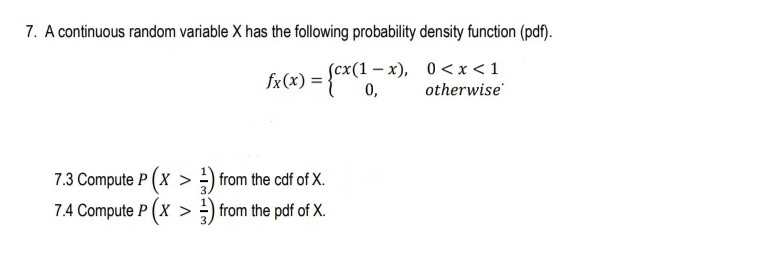
7. A continuous random variable X has the following probability density function (pdf).fx(x) = {AScx(1 – x), 0 -) from the cdf of X.7.4 Compute P (X > ) from the pdf of X.

here calculate constant C using total probability rule then calculate CDF

Answered: 7.3 Compute P (x > ) from the cdf of X.…

MATLAB: An Introduction with Applications

6th Edition

ISBN:9781119256830

Author:Amos Gilat

Publisher:Amos Gilat

Chapter1: Starting With Matlab

Section: Chapter Questions

Problem 1P

See similar textbooks

Similar questions

Suppose that the following import function for Turkey is estimated for Turkey between 1980-2015. In order to measure the impact of 2001 crisis the regression is estimated based on the whole and two subsamples and the following RSS are obtained. Time period: 1980-2000 , RSS1= 69 Time period: 2001-2015, RSS2 =35 Time period: 1980-2015 , RSS = 160 Carry out the Chow test whether the regressions for the two periods are different at 5% significance level.
The variance of temperatures (Fahrenheit) in Mobile, Ala. is 165.16. What is this variance if temp is re-expressed in Celsius? [Hint: Conversion between Fahrenheit and Celsius is a linear transformation: Fahrenheit = Celsius*1.80 + 32, or Celsius = Fahrenheit*(1/1.80) - (32/1.80)]
1.Tukey HSD analysis has the function similar to Duncan MRT analysis.a)Explain on the TWO main function of Tukey HSD analysis. b)Explain on why Tukey HSD analysis not involving any hypothesis.
The variance of temperatures (Fahrenheit) in Buffalo, N.Y. is 362.18. What is this variance if temp is re-expressed in Celsius? [Hint: Conversion between Fahrenheit and Celsius is a linear transformation: Fahrenheit = Celsius*1.80 + 32, or Celsius = Fahrenheit*(1/1.80) - (32/1.80)]
To the Internal Revenue Service (IRS), the reasonableness of total itemized deductions depends on the taxpayer's adjusted gross income. Large deductions, which include charity and medical deductions, are more reasonable for taxpayers with larg given level of income, the chances of an IRS audit are increased. Data (in thousands of dollars) on adjusted gross income and the average or reasonable amount of itemized deductions follow. Adjusted Gross Income Itemized Deductions ($1,000s) 22 ($1,000) 9.6 27 9.6 32 10.1 48 11.1 65 13.5 85 120 15.7 25.5 (a) Develop a scatter diagram for these data with adjusted gross income as the independent variable. 30 25 20 15 10 5 30 25 20 15 10 5+ 30 25- 20- 15- 10- .. 5- 0 20 40 60 80 100 120 140 Adjusted Gross Income ($1,000s) 0 20 40 60 80 100 120 140 0 Adjusted Gross Income ($1,000s) 20 40 60 80 100 120 140 Adjusted Gross Income ($1,000s) 30 25 20 15 10 5- 0 20 40 60 80 100 Adjusted Gross Income ($1,000s) 120 140 G (b) Use the least squares method to…
Suppose that the following import function for Turkey is estimated for Turkey between 1980-2015. In order to measure the impact of 2001 crisis the regression is estimated based on the whole and two subsamples and the following RSS are obtained. Time period: 1980-2000 , RSS1= 69 Time period: 2001-2015, RSS2 =35 Time period: 1980-2015 , RSS = 160 Carry out the Chow test whether the regressions for the two periods are different at 5% significance level.
Suppose that the following import function for Turkey is estimated for Turkey between 1980-2015. In order to measure the impact of 2001 crisis the regression is estimated based on the whole and two subsamples and the following RSS are obtained. Time period: 1980-2000 , RSŠ1= 69 Time period: 2001-2015, RSS2 =35 Time period: 1980-2015 , RSS = 160 Carry out the Chow test whether the regressions for the two periods are different at 5% significance level. %3D
As part of a study at a large university, data were collected on n = 224 freshmen computer science (CS) majors in a particular year. The researchers were interested in modeling y, a student's grade point average (GPA) after three semesters, as a function of the following independent variables (recorded at the time the students enrolled in the university): X 1= average high school grade in mathematics (HSM) X 2 = average high school grade in science (HSS) X 3 = average high school grade in English (HSE) X 4 = SAT mathematics score (SATM) x 5 = SAT verbal score (SATV) A first-order model was fit to the data with the following results: SOURCE DF MS F VALUE PROB>F MODEL 28.64 5.73 11.69 0001 ERROR 218 106 82 0.49 TOTAL 223 135.46 ROOT MSE DEP MEAN 0.700 R-SQUARE 0.211 4.635 ADJ R-SQ 0.193 PARAMETER STANDARD T FOR O VARIABLE ESTIMATE ERROR PARAMETER -0 PROB> ITI INTERCEPT 2.327 0.039 5.817 0.0001 0.0003 XI HSM) X2 (HSS) X3 (HSE) X4 (SATM) X5 (SATV) 0.146 0.037 3.718 a.036 0.038 0.950 0.3432…
For the following table, assume that y = a (x ^b). Then 7 7 11 11 17 13 25 y = 3.083 x^2.312 O y = 2.2083 x^1.04 y = 1.1083 x^1.0945 O y = 2.2 x^1.33 2.
drivers of that Age - ]]], [16 – 17,1,55], [18 - 19,2,30], [20 - 24, 3, A traffic safety organization has compiled data in an urban region of Canada on the rate of non-fatal vehicle injury accidents, y, as a function of the age of the driver, x. The data is shown below. It is assumed that an injury accident affects either the driver or passengers or others external to the vehicle and does not result in death. Age Range of x, Designated Age Driver Category of Driver y, Number of Injury Accidents per 10 million km driven by drivers of that Age 16-17 1 55 18-19 2 30 20-24 3 24 25-29 4 22 30-39 5 14 40-49 6 13 50-59 7 12 60-69 8 10 70-79 9 14 10
In a snow geese feeding trial, a model was constructed relating gosling** weight change (Y), to digestion efficiency (X1) which is measured on a scale from 1 to 10, depending on how well nutrition is absorbed by the goosling, and diet (either plants or duck chow). Using Bi, etc. to represent the coefficients of independent variables, and defining any independent variables you create and use, write out the following: [WRITE OUT THE FULL MODELS IN SINGLE EQUATIONS IN EACH SECTION BELOW, NOT BROKEN DOWN INTO SEPARATE SUB-EQUATIONS] Define your independent variables here a) a first order model that allows for different intercepts but the same slope for each diet b) a first order model that allows for different slopes and intercepts for each diet (c) a first order model that allows for different slopes and the same intercept for each diet
(b) Let X represent the lifetime in months of a certain brand of light bulb. The pdf of X is given by f(x)=K(6-x), 0

SEE MORE QUESTIONS

Recommended textbooks for you

MATLAB: An Introduction with Applications

Statistics

ISBN:

9781119256830

Author:

Amos Gilat

Publisher:

John Wiley & Sons Inc

Probability and Statistics for Engineering and th…

Statistics

ISBN:

9781305251809

Author:

Jay L. Devore

Publisher:

Cengage Learning

Statistics for The Behavioral Sciences (MindTap C…

Statistics

ISBN:

9781305504912

Author:

Frederick J Gravetter, Larry B. Wallnau

Publisher:

Cengage Learning

MATLAB: An Introduction with Applications

Statistics

ISBN:

9781119256830

Author:

Amos Gilat

Publisher:

John Wiley & Sons Inc

Probability and Statistics for Engineering and th…

Statistics

ISBN:

9781305251809

Author:

Jay L. Devore

Publisher:

Cengage Learning

Statistics for The Behavioral Sciences (MindTap C…

Statistics

ISBN:

9781305504912

Author:

Frederick J Gravetter, Larry B. Wallnau

Publisher:

Cengage Learning

Elementary Statistics: Picturing the World (7th E…

Statistics

ISBN:

9780134683416

Author:

Ron Larson, Betsy Farber

Publisher:

PEARSON

The Basic Practice of Statistics

Statistics

ISBN:

9781319042578

Author:

David S. Moore, William I. Notz, Michael A. Fligner

Publisher:

W. H. Freeman

Introduction to the Practice of Statistics

Statistics

ISBN:

9781319013387

Author:

David S. Moore, George P. McCabe, Bruce A. Craig

Publisher:

W. H. Freeman

SEE MORE TEXTBOOKS

7.3 Compute P (x > ) from the cdf of X. 7.4 Compute P (x > |from the pdf of X.