
Introductory Circuit Analysis (13th Edition)
13th Edition
ISBN: 9780133923605
Author: Robert L. Boylestad
Publisher: PEARSON
expand_more
expand_more
format_list_bulleted
Related questions
Concept explainers
Question
answer question in handwriting
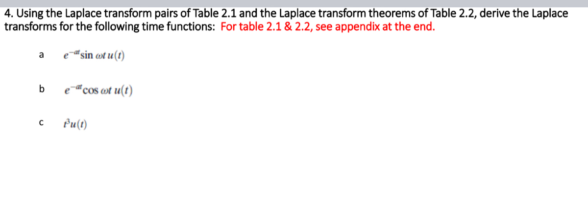

Transcribed Image Text:4. Using the Laplace transform pairs of Table 2.1 and the Laplace transform theorems of Table 2.2, derive the Laplace
transforms for the following time functions: For table 2.1 & 2.2, see appendix at the end.
e-at sin ot u(t)
a
b
с
e-at cos wt u(t)
Bu(t)
![Appendix
TABLE 2.1 Laplace transform table
Item no.
f(1)
1.
2.
3.
4.
5.
6.
7.
1.
2.
3.
4.
5.
6.
TABLE 2.2 Laplace transform theorems
Item no.
Theorem
7.
8.
9.
10.
11.
12.
L[f(t)]=F(s) = f(t)e-sdt
L[kf (1)]
L
8(1)
u(t)
=kF(s)
Lf11) +f2(1)] = F₁(s) + F2(s)
Le-atf(1)]
= F(s+a)
L[f(1-T)]
= e-sTF(s)
L[f(at)] ---F(²)
HESE
tu(t)
t"u(t)
e-at u(t)
sin cotu(t)
cos atu(t)
dt
di
[d"f
den
L[fo_f(t)dt]
f(xo)
ƒ(0+)
F(s)
S
=lim sF(s)
S-0
=lim sF(s)
F(s)
-
1
1
S
1
$2
n!
sh +1
1
s+a
=SF (s)-f(0-)
=s²F(s)- sf (0-) - f'(0-)
=s" F (s)-s-kpk-1 (0-)
k=1
(
s² + w²
S
s²+w²
Name
Definition
Linearity theorem
Linearity theorem
Frequency shift theorem
Time shift theorem
Scaling theorem
Differentiation theorem
Differentiation theorem
Differentiation theorem
Integration theorem
Final value theorem¹
Initial value theorem²
¹For this the orem to yield correct finite results, all roots of the denominator of F(s) must have negative real
parts, and no more than one can be at the origin.
2For this theorem to be valid, f(t) must be continuous or have a step discontinuity at t= 0 (that is, no
impulses or their derivatives at t= 0).](https://content.bartleby.com/qna-images/question/5c85250b-6a52-47e3-86e8-89d741652c47/09c5c760-f9e7-467f-a6a9-75246d3f2ac3/0y5oykn_processed.jpeg)
Transcribed Image Text:Appendix
TABLE 2.1 Laplace transform table
Item no.
f(1)
1.
2.
3.
4.
5.
6.
7.
1.
2.
3.
4.
5.
6.
TABLE 2.2 Laplace transform theorems
Item no.
Theorem
7.
8.
9.
10.
11.
12.
L[f(t)]=F(s) = f(t)e-sdt
L[kf (1)]
L
8(1)
u(t)
=kF(s)
Lf11) +f2(1)] = F₁(s) + F2(s)
Le-atf(1)]
= F(s+a)
L[f(1-T)]
= e-sTF(s)
L[f(at)] ---F(²)
HESE
tu(t)
t"u(t)
e-at u(t)
sin cotu(t)
cos atu(t)
dt
di
[d"f
den
L[fo_f(t)dt]
f(xo)
ƒ(0+)
F(s)
S
=lim sF(s)
S-0
=lim sF(s)
F(s)
-
1
1
S
1
$2
n!
sh +1
1
s+a
=SF (s)-f(0-)
=s²F(s)- sf (0-) - f'(0-)
=s" F (s)-s-kpk-1 (0-)
k=1
(
s² + w²
S
s²+w²
Name
Definition
Linearity theorem
Linearity theorem
Frequency shift theorem
Time shift theorem
Scaling theorem
Differentiation theorem
Differentiation theorem
Differentiation theorem
Integration theorem
Final value theorem¹
Initial value theorem²
¹For this the orem to yield correct finite results, all roots of the denominator of F(s) must have negative real
parts, and no more than one can be at the origin.
2For this theorem to be valid, f(t) must be continuous or have a step discontinuity at t= 0 (that is, no
impulses or their derivatives at t= 0).
Expert Solution
This question has been solved!
Explore an expertly crafted, step-by-step solution for a thorough understanding of key concepts.

This is a popular solution

Trending nowThis is a popular solution!

Step by stepSolved in 2 steps with 3 images

Knowledge Booster


Learn more about
Need a deep-dive on the concept behind this application? Look no further. Learn more about this topic, electrical-engineering and related others by exploring similar questions and additional content below.Similar questions
arrow_back_ios
arrow_forward_ios
Recommended textbooks for you
- Introductory Circuit Analysis (13th Edition)Electrical EngineeringISBN:9780133923605Author:Robert L. BoylestadPublisher:PEARSON
 Delmar's Standard Textbook Of ElectricityElectrical EngineeringISBN:9781337900348Author:Stephen L. HermanPublisher:Cengage Learning
 Programmable Logic ControllersElectrical EngineeringISBN:9780073373843Author:Frank D. PetruzellaPublisher:McGraw-Hill Education
  Fundamentals of Electric CircuitsElectrical EngineeringISBN:9780078028229Author:Charles K Alexander, Matthew SadikuPublisher:McGraw-Hill Education
 Electric Circuits. (11th Edition)Electrical EngineeringISBN:9780134746968Author:James W. Nilsson, Susan RiedelPublisher:PEARSON
 Engineering ElectromagneticsElectrical EngineeringISBN:9780078028151Author:Hayt, William H. (william Hart), Jr, BUCK, John A.Publisher:Mcgraw-hill Education,
Introductory Circuit Analysis (13th Edition)
Electrical Engineering
ISBN:9780133923605
Author:Robert L. Boylestad
Publisher:PEARSON
Delmar's Standard Textbook Of Electricity
Electrical Engineering
ISBN:9781337900348
Author:Stephen L. Herman
Publisher:Cengage Learning
Programmable Logic Controllers
Electrical Engineering
ISBN:9780073373843
Author:Frank D. Petruzella
Publisher:McGraw-Hill Education
Fundamentals of Electric Circuits
Electrical Engineering
ISBN:9780078028229
Author:Charles K Alexander, Matthew Sadiku
Publisher:McGraw-Hill Education
Electric Circuits. (11th Edition)
Electrical Engineering
ISBN:9780134746968
Author:James W. Nilsson, Susan Riedel
Publisher:PEARSON
Engineering Electromagnetics
Electrical Engineering
ISBN:9780078028151
Author:Hayt, William H. (william Hart), Jr, BUCK, John A.
Publisher:Mcgraw-hill Education,