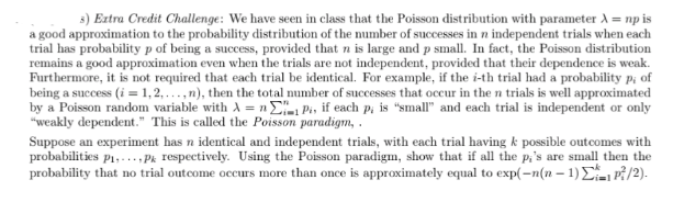
3) Extra Credit Challenge: We have seen in class that the Poisson distribution with parameter A = np is a good approximation to the probability distribution of the number of successes in n independent trials when each trial has probability p of being a success, provided that n is large and p small. In fact, the Poisson distribution remains a good approximation even when the trials are not independent, provided that their dependence is weak. Furthermore, it is not required that each trial be identical. For example, if the i-th trial had a probability p; of being a success (i =1, 2,...,n), then the total number of successes that occur in the n trials is well approximated by a Poisson random variable with A = n E, Pi, if each Pi is "small" and each trial is independent or only "weakly dependent." This is called the Poisson paradigm, . Suppose an experiment has n identical and independent trials, with each trial having k possible outcomes with probabilities p1,..., Pk respectively. Using the Poisson paradigm, show that if all the p;'s are small then the probability that no trial outcome occurs more than once is approximately equal to exp(-n(n – 1) E=, P /2).

I need the answer as soon as possible

Aa.127.   Let X1,X2,...,X4 be indepedent Poisson random variables with rates λ1,...,λ4, respectively. Show that X1 + X2 + X3 + X4 is a Poisson random variable with rate λ1 + λ2 + λ3 + λ4.

A statistics professor finds that when he schedules an office hour at the 10:30 a.m. time slot, an average of three students arrives. Use the Poisson distribution to find the probability that in a randomly selected office hour no students will arrive. O A. 0.1225 O B. 0.0743 O C. 0.1108 O D. 0.0498 O Time Remaining: 01:08:58 Next TCJT 11 Test 2 1-45 of 45

9. This is a simplified inventory problem. Suppose that it costs c dollars to stock anitem and that the item sells for s dollars. Suppose that the number of items thatwill be asked for by customers is a random variable with the frequency functionp(k). Find a rule for the number of items that should be stocked in order tomaximize the expected income. (Hint: Consider the difference of successiveterms.)

A barbershop is operated by one barber and has a space capacity to accommodate for a total of 6 customers (including the one in service). If a customer comes to this shop and finds it full, he goes to other shops. Customers arrive according to Poisson distribution at a rate of 4.1 customers per hour. The barber’s service time is exponential and he can serve at a rate of 7.1 customers per hour. a. What is the probability that the barber is free? Answer = Answer b. What is the expected number of people in the system? Answer = Answer c. What is the expected waiting time in the queue? Answer = Answerhours. (hint: use effective arrival rate)

The data records the smiling times, in seconds, of an eight-week-old baby.We will assume that the smiling times, in seconds, follow a uniform distribution between zero and 23 seconds, inclusive. This means that any smiling time from zero to and including 23 seconds is equally likely.What is the probability that a randomly chosen eight- week-old baby smiles between two and 18 seconds? O 0.1304 O 0.8696 O 0.6957 0.7826