
Advanced Engineering Mathematics
10th Edition
ISBN: 9780470458365
Author: Erwin Kreyszig
Publisher: Wiley, John & Sons, Incorporated
expand_more
expand_more
format_list_bulleted
Related questions
Question
21,25

Transcribed Image Text:First-Order Differential Equations
b. Explain why the existence of two solutions of the
Theorem 2.4.2.
given problem does not contradict the uniqueness part of
c. Show that y = ct + c², where c is an arbitrary constant,
satisfies the differential equation in part a fort 2-2c. If c = -1,
the initial condition is also satisfied, and the solution y = y₁ (1) is
solution y = y₂(t).
obtained. Show that there is no choice of c that gives the second
19. a. Show that (t) = e2¹ is a solution of y' - 2y = 0 and that
y = co(t) is also a solution of this equation for any value of the
constant c.
b. Show that (t) = 1/t is a solution of y' + y2 = 0 for t > 0,
but that y = co(t) is not a solution of this equation unless c = 0
of part a is linear.
or c = 1. Note that the equation of part b is nonlinear, while that
20. Show that if y = (t) is a solution of y' + p(t) y = 0, then
y = co(t) is also a solution for any value of the constant c.
21. Let y = y₁ (t) be a solution of
y' + p(t) y = 0,
and let y = y₂(t) be a solution of
tomize
y' + p(t) y = g(t).
where c is an arbitrary constant.
b. Show that y₁ is a solution of the differential equation
y' + p(t) y = 0,
Show that y = y₁ (t) + y2(t) is also a solution of equation (28).
can be written in the form
22. a. Show that the solution (7) of the general linear equation (1)
y = cy₁ (t) + y₂(t),
y' + p(t)y=q(t) y",
(27)
corresponding to g(t) = 0.
c. Show that y2 is a solution of the full linear equation (1). We
see later (for example, in Section 3.5) that solutions of higher-
order linear equations have a pattern similar to equation (29).
ernoulli Equations. Sometimes it is possible to solve a nonlinear
mation by making a change of the dependent variable that converts
nto a linear equation. The most important such equation has the
m
SKITO
melding
(29)
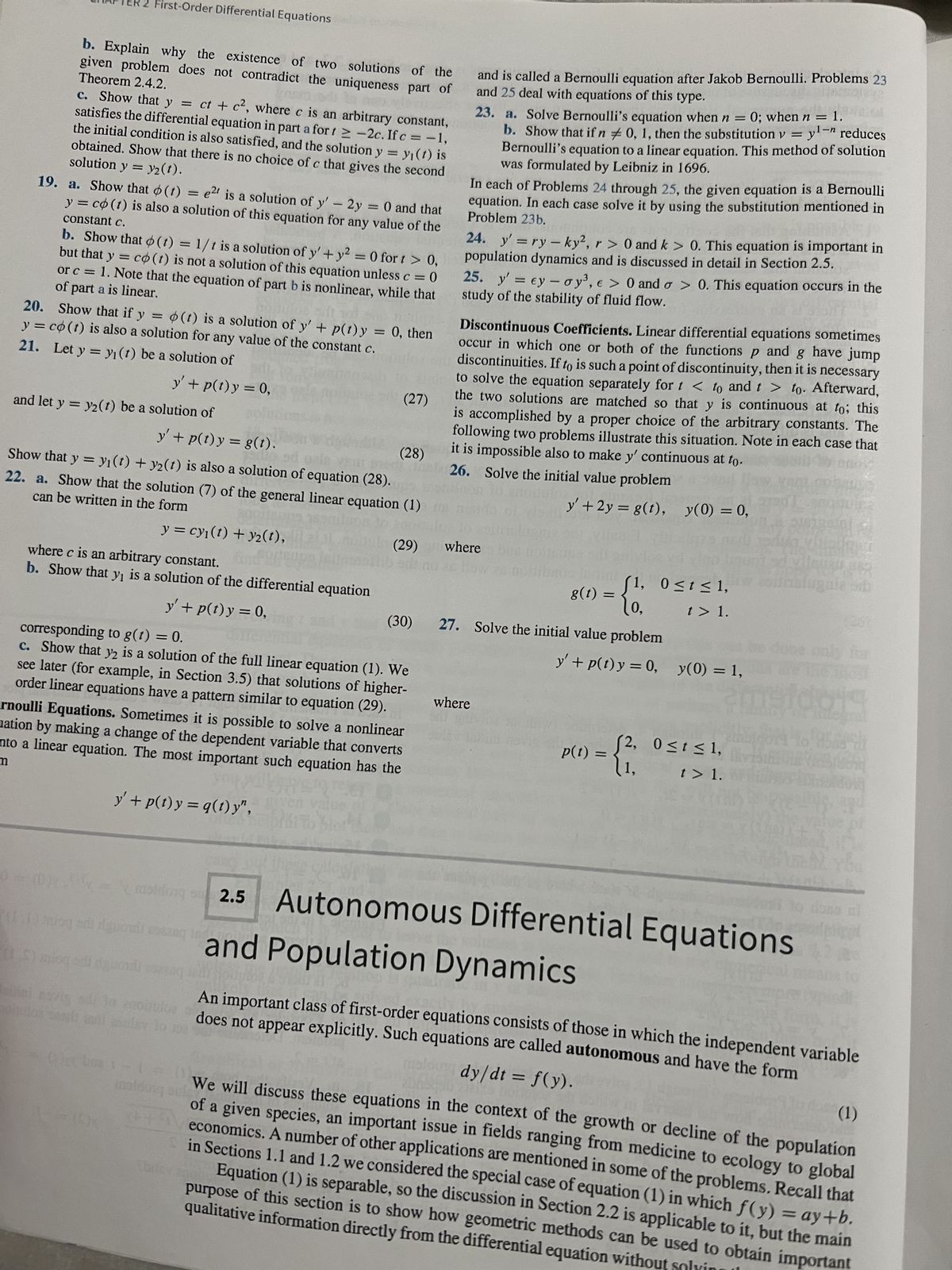
Discontinuous Coefficients. Linear differential equations sometimes
occur in which one or both of the functions p and g have jump
discontinuities. If to is such a point of discontinuity, then it is necessary
to solve the equation separately for t < to and t > to. Afterward,
the two solutions are matched so that y is continuous at to; this
is accomplished by a proper choice of the arbitrary constants. The
following two problems illustrate this situation. Note in each case that
(28)
it is impossible also to make y' continuous at to.
dani 26. Solve the initial value problem
y' + 2y = g(t), y(0) = 0,
212501
and is called a Bernoulli equation after Jakob Bernoulli. Problems 23
and 25 deal with equations of this type.
201
23. a. Solve Bernoulli's equation when n = 0; when n = 1.
b. Show that if n 0, 1, then the substitution v = yl-n reduces
Bernoulli's equation to a linear equation. This method of solution
was formulated by Leibniz in 1696.
In each of Problems 24 through 25, the given equation is a Bernoulli
equation. In each case solve it by using the substitution mentioned in
Problem 23b.
24. y'=ry - ky2, r> 0 and k > 0. This equation is important in
population dynamics and is discussed in detail in Section 2.5.
25. y' = ey- oy³, e > 0 and a > 0. This equation occurs in the
study of the stability of fluid flow.
where
Iton
where
sau par
g(t) =
(30) 27. Solve the initial value problem
= {1; 05
(0)
(1) miog dirigenti ea and Population Dynamics
(1) mloq adi dauond
0≤t≤ 1,
P(1) = {};
y' + p(t) y = 0, y(0) = 1,
t > 1.
villausu geg
unalugnie od
ameldolg
0 ≤ t ≤ 1,
t > 1.
(12-18 1²
molding ou 2.5
2.5 Autonomous Differential Equations
An important class of first-order equations consists of those in which the independent variable
does not appear explicitly. Such equations are called autonomous and have the form
dy/dt = f(y).
(1)
We will discuss these equations in the context of the growth or decline of the population
of a given species, an important issue in fields ranging from medicine to ecology to global
economics. A number of other applications are mentioned in some of the problems. Recall that
in Sections 1.1 and 1.2 we considered the special case of equation (1) in which f(y) = ay+b.
Equation (1) is separable, so the discussion in Section 2.2 is applicable to it, but the main
qualitative information directly from the differential equation without
purpose of this section is to show how geometric methods can be used to obtain important
Expert Solution
This question has been solved!
Explore an expertly crafted, step-by-step solution for a thorough understanding of key concepts.

This is a popular solution

Trending nowThis is a popular solution!

Step by stepSolved in 2 steps with 2 images

Knowledge Booster

Recommended textbooks for you
- Advanced Engineering MathematicsAdvanced MathISBN:9780470458365Author:Erwin KreyszigPublisher:Wiley, John & Sons, Incorporated
 Numerical Methods for EngineersAdvanced MathISBN:9780073397924Author:Steven C. Chapra Dr., Raymond P. CanalePublisher:McGraw-Hill Education
 Introductory Mathematics for Engineering Applicat...Advanced MathISBN:9781118141809Author:Nathan KlingbeilPublisher:WILEY
  Mathematics For Machine TechnologyAdvanced MathISBN:9781337798310Author:Peterson, John.Publisher:Cengage Learning,

Advanced Engineering Mathematics
Advanced Math
ISBN:9780470458365
Author:Erwin Kreyszig
Publisher:Wiley, John & Sons, Incorporated
Numerical Methods for Engineers
Advanced Math
ISBN:9780073397924
Author:Steven C. Chapra Dr., Raymond P. Canale
Publisher:McGraw-Hill Education
Introductory Mathematics for Engineering Applicat...
Advanced Math
ISBN:9781118141809
Author:Nathan Klingbeil
Publisher:WILEY
Mathematics For Machine Technology
Advanced Math
ISBN:9781337798310
Author:Peterson, John.
Publisher:Cengage Learning,