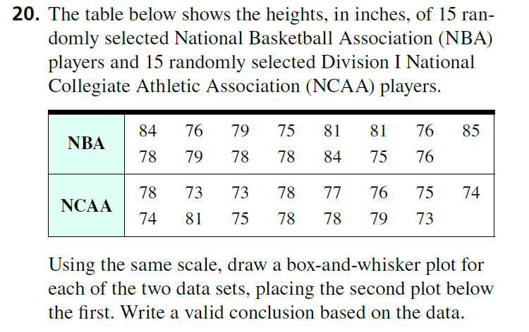
20. The table below shows the heights, in inches, of 15 ran- domly selected National Basketball Association (NBA) players and 15 randomly selected Division I National Collegiate Athletic Association (NCAA) players. 84 76 79 75 81 81 76 85 NBA 78 79 78 78 84 75 76 78 73 73 78 77 76 75 74 NCAA 74 81 75 78 78 79 73 Using the same scale, draw a box-and-whisker plot for each of the two data sets, placing the second plot below

None

regression, econometrics

The next 3 questions refer to the following: A housecleaning company receives 36 for each house cleaned. The tab below gives the relation between the number of workers and the number houses that can be cleaned per week. [[[[ Number of], [Workers]], [[Houses], [Cleaned]]], [0, 0], [1, 9], [2, 17], [3, 24], [4, 30], [5, 35], [6,36]] The marginal revenue from the fourth worker is If the company want to maximize profit and hires three workers, the wa rate of a house - cleaner can be no more than If the wage rate of a house - cleaner is 140, the maximum amount of pr the company can earn is

a) What is a Z score? Explain. b) A data value of Z score -1. What is the relative position of the data value? Explain.

Martha’s Wonderful Cookie Company makes a specialsuper chocolate-chip peanut butter cookie. The companywould like the cookies to average approximately eightchocolate chips apiece. Too few or too many chips distortthe desired cookie taste. Twenty samples of five cookieseach during a week have been taken and the chocolatechips counted. The sample observations are as follows: Construct an -chart in conjunction with an R-chart using 3 limits for this data and comment on the cookie-production process. Samples Chips per Cookie1 7 69 852 7 7 8 8 103 5 57 684 4 59 97

We have estimated the impact of gross domestic product (GDP), energy consumption (ENERGY) and population (POP) on CO2 emiisions (CO2) in Cyprus. The results are as follows, Dependent Variable: CO2 Method: Least Squares Date: 04/20/17 Time: 09.46 Sample: 1990 2013 Included observations: 24 Variable Coefficient Std. Error t-Statistic Prob. GDP ENERGY POP 2.002813 0.022114 -0.734352 0.203927 6.458672 0.011872 0.328388 0.293686 0,310097 1.862670 -2.236233 0.694371 0.7597 0.0773 0,0369 0.4954 R-squared Adjusted R-squared S.E. of regression Sum squared resid Log likelihood F-statistic Prob(F-statistic) 0.825079 Mean dependentyar 0.798841 0.048515 Akaike info criterion 0.047074 Schwarz criterion 40.75460 Hannan-Quinn.criter. 31.44583 Durbin-Wats on stat 0.000000 3.625982 0.108170 -3.062883 -2.866541 -3.010793 1.410912 S.D. dependent yar a Write down the economie function for the above estimation by using the information obtained from above table| b- Write down the economic model for the above…

Researchers conducted an observational study of automobile drivers and their cell phone use by manually observing traffic in heavily congested areas. They would record the amount of time they observed individual drivers on the phone while operating their vehicle in stop and go traffic and the number of accidents on a particular section of highway over the course of a month. The accompanying graph depict the data they recorded, each point represents a 1 mile section of heavily congested roads. From the data, which of these is a potentially valid conclusion? Cell-phone use while driving increases the rate of accidents. O Car accidents and cell-phone use have no relationship. The increasing rate of car accidents causes increased phone-call length. A conclusion cannot be made; the data ignores the omitted variable of which cell-phone provider each person uses. If the x and y variables were swapped, what would the new slope be? zero positive Number of car accidents 10- 9- 8- 7- 5- 4- 3- 2-…

Find out the coefficient of Variation (CV). Please discuss the effect of large observation with the help of CV. Use MS-EXCEL for the Calculation, Take Snapshot after analysis and paste it

2. To help determine how many beers to stock the concession manager at Yankee Stadium wanted to know how the temperature affected beer sales. Accordingly, she took a sample of 10 games and recorded the number of beers sold and the temperature in the middle of the game. Temperature 80 68 78 79 87 Number of 20,533 1,439 13,829 21,286 30,985 beers Temperature 74 86 92 77 84 Number of 17,187 30,240 37,596 9,610 28,742 beers a. Predict with 90% confidence the number of beers to be sold when temperature is 75 degrees. b. Calculate and plot the residuals and predicted values of y.