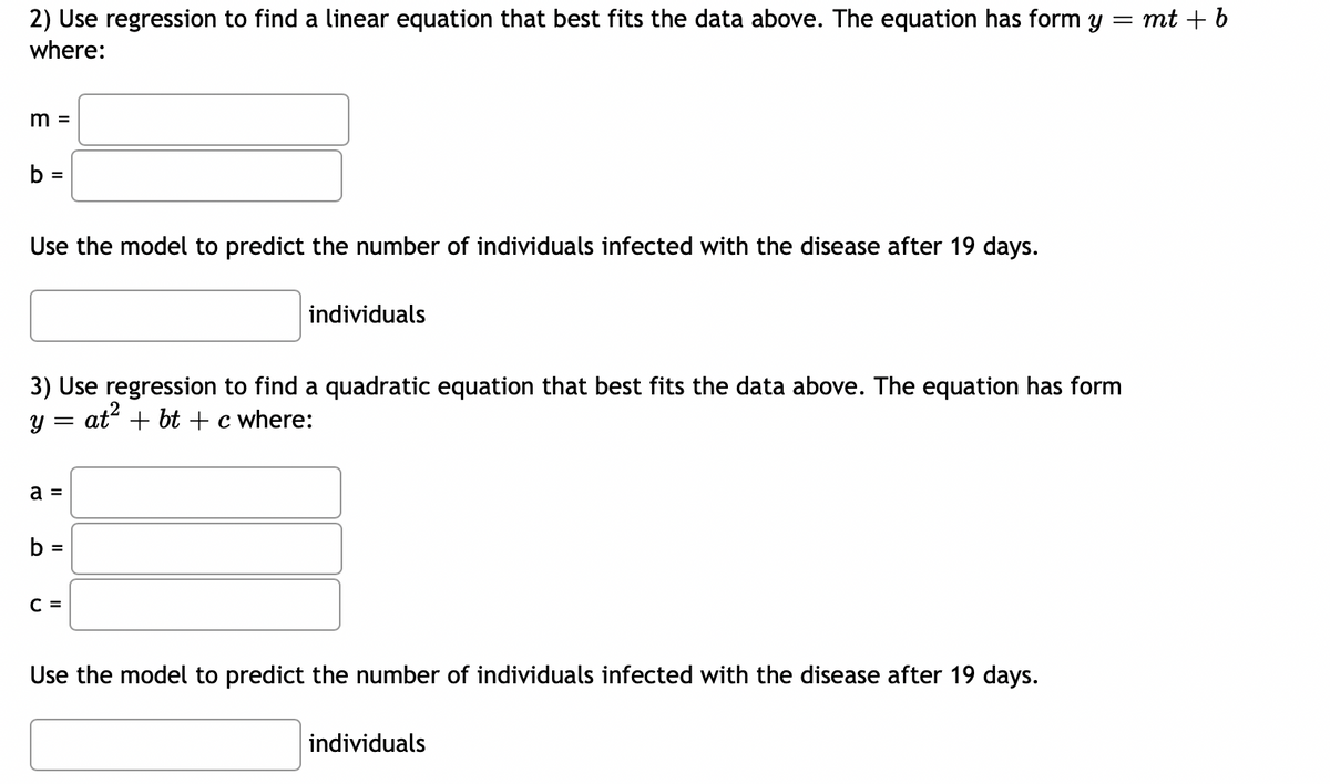
2) Use regression to find a linear equation that best fits the data above. The equation has form y = mt + b where: m = b = Use the model to predict the number of individuals infected with the disease after 19 days. 3) Use regression to find a quadratic equation that best fits the data above. The equation has form y = at² + bt + c where: a = b = individuals C = Use the model to predict the number of individuals infected with the disease after 19 days. individuals

The volume​ (in cubic​ feet) of a black cherry tree can be modeled by the equation y=−50.8+0.3x1+5.1x2​, where x1 is the​ tree's height​ (in feet) and x2 is the​ tree's diameter​ (in inches). Use the multiple regression equation to predict the​ y-values for the values of the independent variables.

The volume​ (in cubic​ feet) of a black cherry tree can be modeled by the equation y=−51.9+0.3x1+4.9x2​, where x1 is the​ tree's height​ (in feet) and x2 is the​ tree's diameter​ (in inches). Use the multiple regression equation to predict the​ y-values for the values of the independent variables.

A professor wants to predict students' final examination scores on the basis of their midterm test scores. An equation was determined on the basis of data on the scores of three students who took the same course with the same instructor the previous semester (see the table on the right). a) Find the regression line, y=mx+b. Midterm Score, x 82 65 69 Final Exam Score, y b)The midterm score of a student was 88%. Use the regression line to predict the student's final exam score. 87 67 78 a) y = ☐ (Simplify your answer. Round to five decimal places as needed.) b) The student's final exam score is (Simplify your answer. Round to two decimal places as needed.).

***PLEASE INCLUDE EXCEL OUTPUT WITH YOUR RESPONSE

A study tests the effect of earning a Master's degree on the salaries of professionals. Suppose that the salaries of the professionals (S,) are not dependent on any other variables. Let D, be a variable which takes the value 0 if an individual has not earned a Master's degree, and a value 1 if they have earned a Master's degree. What would be the regression model that the researcher wants to test? A. S,= Po + B,D,+u, i=1, .. , n. O B. S,= Po + B, + u, i= 1, .. , n. OC. 1=6o +B1,S, + u, i= 1, .. , n. O D. 0=Bo +B, S, + u,, i= 1, .. , n. Suppose that a random sample of 160 individuals suggests that professionals without a Master's degree earn an average salary of $59,000 per annum, while those with a Master's degree earn an average salary of $80,000 per annum. The OLS estimate of the coefficient B, will be $ and that of B, will be $ Click to select your answer(s). DELL

The volume (in cubic feet) of a black cherry tree can be modeled by the equation y = - 50.8 + 0.3x, +4.5x,, where x, is the tree's height (in feet) and x, is the tree's diameter (in inches). Use the multiple regression equation to predict the y-values for the values of the independent variables. x, = 70, x, = 8.6 The predicted volume is cubic feet. (Round to one decimal place as needed.)