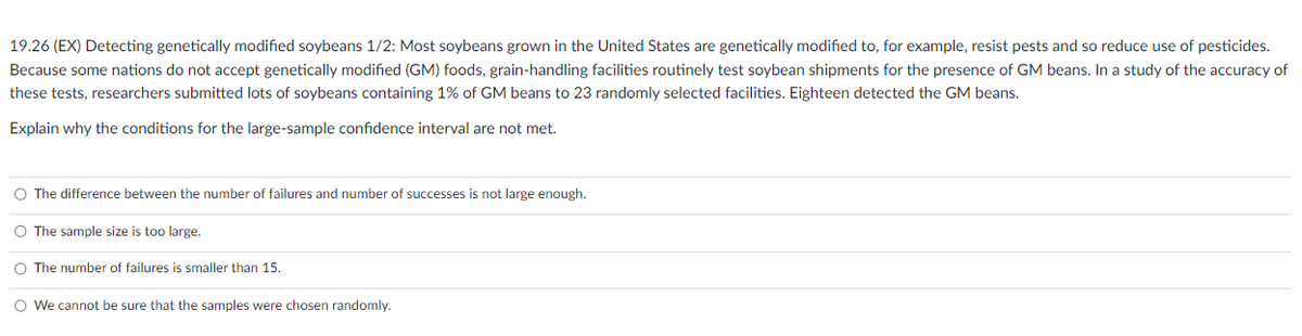
19.26 (EX) Detecting genetically modified soybeans 1/2: Most soybeans grown in the United States are genetically modified to, for example, resist pests and so reduce use of pesticides. Because some nations do not accept genetically modified (GM) foods, grain-handling facilities routinely test soybean shipments for the presence of GM beans. In a study of the accuracy of these tests, researchers submitted lots of soybeans containing 1% of GM beans to 23 randomly selected facilities. Eighteen detected the GM beans. Explain why the conditions for the large-sample confidence interval are not met. O The difference between the number of failures and number of successes is not large enough. O The sample size is too large. O The number of failures is smaller than 15. O We cannot be sure that the samples were chosen randomly.

In a lake pollution study, the concentration of lead in the upper sedimentary layer of a lake bottom is measured from 25 sediment samples. The sample mean and the standard deviation of the measurements are found to be 0.38 and 0.06, respectively. Suppose Ho : u = 0.34 H1: u# 0.34 (a) State Type I and Type Il errors. (b) Conduct a hypothesis test at 0.01 level of significance by doing the seven-step classical approach. (please show all seven steps, formulas, calculations and the curve)

Test whether mu 1 less than mu 2μ1<μ2 at the alphaα=0.01 level of significance for the sample data shown in the accompanying table. Assume that the populations are normally distributed.   Determine the null and alternative hypothesis for this test.     A. H0:mu 1<mu 2μ1<μ2 H1:mu 1= mu 2μ1=μ2   B. Upper H 0 :H0:mu 1 equals mu 2μ1=μ2 Upper H 1 :H1:mu 1 not equals mu 2μ1≠μ2   C. Upper H 0 :H0:mu 1 not equals mu 2μ1≠μ2 Upper H 1 :H1:mu 1 less than mu 2μ1<μ2   D. Upper H 0 :H0:mu 1 equals mu 2μ1=μ2 Upper H 1 :H1:mu 1 less than mu 2μ1<μ2 Your answer is correct.   Detemine the​ P-value for this hypothesis test.   Pequals=nothing ​(Round to three decimal places as​ needed.)

A newly installed automatic gate system was being tested to see if the number of failures in 1,000 entry attempts was the same as the number of failures in 1,000 exit attempts. A random sample of eight delivery trucks was selected for data collection. Do these sample results show that there is a significant difference between entry and exit gate failures? Use α = 0.05.    Truck 1 Truck 2 Truck 3 Truck 4 Truck 5 Truck 6 Truck 7 Truck 8 Entry failures 44 42 53 56 62 53 48 43 Exit failures 48 50 55 60 57 48 50 48  Click here for the Excel Data File (b) Find the test statistic tcalc. (Round your answer to 3 decimal places. A negative value should be indicated by a minus sign.)      (c) Find the critical value tcrit for α = 0.05. (Round your answer to 3 decimal places. A negative value should be indicated by a minus sign.)      (d) Find the p-value. (Round your answer to 4 decimal places.)      (e) State your conclusion.                           Automated Gate: Number of…