MATLAB: An Introduction with Applications
6th Edition
ISBN: 9781119256830
Author: Amos Gilat
Publisher: John Wiley & Sons Inc
expand_more
expand_more
format_list_bulleted
Question

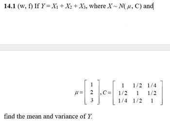
Transcribed Image Text:14.1 (w, f) If Y= X₁ + X₂ + X3, where X~ N(μ, C) and
1
----
=
2
3
find the mean and variance of Y.
1 1/2 1/4
1 1/2
1/2
1/4 1/2 1
Expert Solution
This question has been solved!
Explore an expertly crafted, step-by-step solution for a thorough understanding of key concepts.
Step by stepSolved in 2 steps with 2 images

Knowledge Booster
Similar questions
- Suppose that X1,..., X, is a random sample from a normal distribution with mean u and variance o?. Two unbiased estimators of o? are ởf = s° = E(x, - Xy°, and ô = (X1 - 2 Find the efficiency of ở relative to ôž.arrow_forward12) A metal bar is heated, and then allowed to cool. Its temperature T (in °C) is found to be The time is in minutes. T=15+75e-0.25 t Find the time rate of change of temperature after 5.0 minutes. 13) The standard normal curve (sometimes called the bell curve) in statistics looks like: 1 -x² y = e 2 √2π Show that there are two inflection points at x = +1arrow_forward1.9.18. Find the mean and the variance of the distribution that has the cdf x <0 0arrow_forward3.7. Consider the performance function Y = 3x1-2x2 where Xi and X2 are both normally distributed random variables with Ax' = 16.6 0% 2.45 μΧ2 = 18.8 ơx.-2.83 The two variables are correlated, and the covariance is equal to 2.0. Determine the probability of failure if failure is defined as the state when Y 0 3.8. The resistance (or capacity) R of a member is to be modeled using R = R,MPF where Rn is the nominal value of the capacity determined using code procedures and M, P, and Fare random variables that account for various uncertainties in the capacity. If M, P, and F are all lognormal random variables, determine the mean and variance of R in terms of the means and variances of M, P, and F.arrow_forwardN= 150 observations were collected on a time series that was identified as a AR(2) time series. The following statistics were computed from the data. Mean - 45.0 Variance 15.6 Autocorrelation function (up to lag 5) r1 = 0.80, r2 = .50, rз = .26, r4 = -.10, rs = 0.08: == Estimate the parameters of the model using the method of moments.arrow_forwardI need help with parts a and barrow_forwardEL 466 416 13.) The continuous random variable (RV) X is uniform over [0,1). Given Y = -ln X what is P({0arrow_forward18. Because ethanol contains less energy than gasoline, a researcher wants to determine if the mileage of a car (y) is affected by the percent ethanol in the gasoline (x). The true population regression line relating the mean mileage y for a given ethanol content x (in percent) is μy|x = β0 + β1x. In a controlled environment, the mileage of a car is recorded when refueled 7 times using between 0% and 10% ethanol. The least squares regression line was found to be yˆ = βˆ0 + βˆ1x = 32.96 − 0.250x. We wish to test H0 : β1 = 0 versus Ha : β1 < 0 at the α = 0.05 significance level (i.e. we want to determine if the addition of ethanol significantly decreases mean gas mileage). What is the p−value for this test? What is your conclusion? Note: s?e(βˆ1) = 0.0485. Which of the following is/are true? (A) In reference to question (18), it would be appropriate to approximate the mean mileage when the car is using 85% ethanol (B) In reference to question (18), a 95% confidence interval for β1…arrow_forwardarrow_back_iosarrow_forward_iosRecommended textbooks for you
 MATLAB: An Introduction with ApplicationsStatisticsISBN:9781119256830Author:Amos GilatPublisher:John Wiley & Sons Inc
 Probability and Statistics for Engineering and th...StatisticsISBN:9781305251809Author:Jay L. DevorePublisher:Cengage Learning
 Statistics for The Behavioral Sciences (MindTap C...StatisticsISBN:9781305504912Author:Frederick J Gravetter, Larry B. WallnauPublisher:Cengage Learning
 Elementary Statistics: Picturing the World (7th E...StatisticsISBN:9780134683416Author:Ron Larson, Betsy FarberPublisher:PEARSON
 The Basic Practice of StatisticsStatisticsISBN:9781319042578Author:David S. Moore, William I. Notz, Michael A. FlignerPublisher:W. H. Freeman
 Introduction to the Practice of StatisticsStatisticsISBN:9781319013387Author:David S. Moore, George P. McCabe, Bruce A. CraigPublisher:W. H. Freeman
 MATLAB: An Introduction with ApplicationsStatisticsISBN:9781119256830Author:Amos GilatPublisher:John Wiley & Sons Inc
 Probability and Statistics for Engineering and th...StatisticsISBN:9781305251809Author:Jay L. DevorePublisher:Cengage Learning
 Statistics for The Behavioral Sciences (MindTap C...StatisticsISBN:9781305504912Author:Frederick J Gravetter, Larry B. WallnauPublisher:Cengage Learning
 Elementary Statistics: Picturing the World (7th E...StatisticsISBN:9780134683416Author:Ron Larson, Betsy FarberPublisher:PEARSON
 The Basic Practice of StatisticsStatisticsISBN:9781319042578Author:David S. Moore, William I. Notz, Michael A. FlignerPublisher:W. H. Freeman
 Introduction to the Practice of StatisticsStatisticsISBN:9781319013387Author:David S. Moore, George P. McCabe, Bruce A. CraigPublisher:W. H. Freeman