
MATLAB: An Introduction with Applications
6th Edition
ISBN: 9781119256830
Author: Amos Gilat
Publisher: John Wiley & Sons Inc
expand_more
expand_more
format_list_bulleted
Related questions
Question
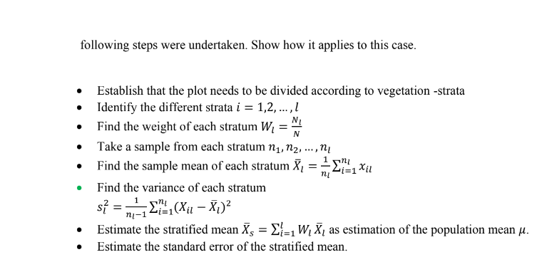

Transcribed Image Text:following steps were undertaken. Show how it applies to this case.
Establish that the plot needs to be divided according to vegetation -strata
●
Identify the different strata i = 1,2,..., l
N₁
Find the weight of each stratum W₂
=
N
•
***
Take a sample from each stratum n₁, №₂,
Find the sample mean of each stratum X₁
,n₂
•
=
I mi
i=1 Xil
ni
●
Find the variance of each stratum
s} =
=7₁-1/²/²1 (X ₁₁ - X₁) ²
Estimate the stratified mean ø = Σ₁=₁ W₁ X, as estimation of the population mean µ.
Estimate the standard error of the stratified mean.

Transcribed Image Text:1.7. Refer to information in 1.6 The one-hectare plot has different types of vegetation - shady areas,
sunny areas. The researchers want to establish whether the type of vegetation has an influence on
the mean height of the flower. They noticed that the two areas are more or less the same size and
the plants were spread evenly over the two areas. Recall the assumption of 1200 plants on this
1 hectare plot. The researchers decide to investigate the shady and the sunny areas in order to
evaluate the mean heights as well record the number of flowering and non-flowering plants. A
sample of 20 plants was taken from the sunny area and a sample of 25 from the shady area. The
mean heights were 85 mm and 75 mm respectively and variances, 4 and 6 respectively. The
Expert Solution
This question has been solved!
Explore an expertly crafted, step-by-step solution for a thorough understanding of key concepts.

Step by stepSolved in 2 steps

Knowledge Booster

Similar questions
- Question 8 Use the following data to identily the box and whisker plot: 48, 47, 16, 31, 26, 40, 11, 23, 50, 18, 42, 49, 19, 25, 10 Your answer: 10 20 30 40 10 20 30 40 50 10 20 30 40 50 10 20 30 40 50arrow_forwardUsing the following stem & leaf plot, find the five number summary for the data by hand. 1|01 2 166 3|16 41 349 5122478 6 14 Min = 10 o Q1 = 41 Med = 37 Q3 = 76 Max = 64 X X Xarrow_forwardConsider the following ordered data. 2 5 5 6 7 7 8 9 10 (a) Find the low, Q1, median, Q3, and high. low Q1 median Q3 high (b) Find the interquartile range.(c) Make a box-and-whisker plot.arrow_forward
- q26- Which of the following charts shows the five numbers summarising the distribution of a variable in a dataset? a. A boxplot b. A histogram c. A cumulative histogram d. A scatter plotarrow_forwardMatch the best graphic to be used for each scenario. To compare the choleterol levels between males and females v [ Chopse] box plot pie chart side by side box plot To display the breakdown of diet types (vegan, vegetarian, low carb, low fat)fat stem plot To describe the distribution of fasting blood [ Choose ] sugar levels among elderly diabetic patients To calculate the proportion of people in a study sample who weigh less than the [Choose] sample meanhah No new data to save. Last checked MacBook Airarrow_forwardB) has more than one answer .. Thank youarrow_forward
- Given the following box plot: 10 12 Determine the following: a. Min = b. Q1 = c. Median = d. Q3 = е. Мах - f. IQR = Q3 - Q1 = g. Range h. Which quarter has the smallest spread of data? 1st 2nd | 3rd 4th i. Which quarter has largest spread of data? 1st 2nd 3rd | 4th j. The percentage of data between the values 2 and 12. 0% |25% O 50% O75% O 100% k. The percentage of data between the values 12 and 13. 0% | 25% 50% 75% 100% O O O 0 O O 0 0arrow_forwardThis is only one questionarrow_forwardA sample of blood pressure measurements is taken from a data set and those values (mm Hg) are listed below. The values are matched so that subjects each have systolic and diastolic measurements. Find the mean and median for each of the two samples and then compare the two sets of results. Are the measures of center the best statistics to use with these data? What else might be better? Systolic: 107 114 101 149 115 121 104 160 112 1500 Diastolic: 88 77 55 61 58 86 66 85 60 82 --..- Find the means. The mean for systolic is| mm Hg and the mean for diastolic is mm Hg. (Type integers or decimals rounded to one decimal place as needed.)arrow_forward
arrow_back_ios
SEE MORE QUESTIONS
arrow_forward_ios
Recommended textbooks for you
- MATLAB: An Introduction with ApplicationsStatisticsISBN:9781119256830Author:Amos GilatPublisher:John Wiley & Sons Inc
 Probability and Statistics for Engineering and th...StatisticsISBN:9781305251809Author:Jay L. DevorePublisher:Cengage Learning
 Statistics for The Behavioral Sciences (MindTap C...StatisticsISBN:9781305504912Author:Frederick J Gravetter, Larry B. WallnauPublisher:Cengage Learning
  Elementary Statistics: Picturing the World (7th E...StatisticsISBN:9780134683416Author:Ron Larson, Betsy FarberPublisher:PEARSON
 The Basic Practice of StatisticsStatisticsISBN:9781319042578Author:David S. Moore, William I. Notz, Michael A. FlignerPublisher:W. H. Freeman
 Introduction to the Practice of StatisticsStatisticsISBN:9781319013387Author:David S. Moore, George P. McCabe, Bruce A. CraigPublisher:W. H. Freeman
MATLAB: An Introduction with Applications
Statistics
ISBN:9781119256830
Author:Amos Gilat
Publisher:John Wiley & Sons Inc
Probability and Statistics for Engineering and th...
Statistics
ISBN:9781305251809
Author:Jay L. Devore
Publisher:Cengage Learning
Statistics for The Behavioral Sciences (MindTap C...
Statistics
ISBN:9781305504912
Author:Frederick J Gravetter, Larry B. Wallnau
Publisher:Cengage Learning
Elementary Statistics: Picturing the World (7th E...
Statistics
ISBN:9780134683416
Author:Ron Larson, Betsy Farber
Publisher:PEARSON
The Basic Practice of Statistics
Statistics
ISBN:9781319042578
Author:David S. Moore, William I. Notz, Michael A. Fligner
Publisher:W. H. Freeman
Introduction to the Practice of Statistics
Statistics
ISBN:9781319013387
Author:David S. Moore, George P. McCabe, Bruce A. Craig
Publisher:W. H. Freeman