1. The linearization at a = 0 to v8+ &x is A + Bx. Compute A and B. %3D A = 2. The linearization at a = 0 to sin(3x) is A + Bx. Compute A and B. A = B 3. Find the linearization L(x) of the function g(x) =xf(x²) at x = 2 given the following infor-mation. f (2) = -1f'(2) = 12f (4) = 6 f'(4) = -2 Answer: L(x) =. 4. The figure below shows f(x) and its local linearization at x = a, y = 3x – 1. (The local linearization is shown in blue.) What is the value of a? a = What is the value of f(a)? f(a) =- Use the linearization to approximate the value of f(2.5). f(2.5) = Is the approximation an under- or overestimate? (Enter under or over.) 5. The figure shows how a function f(x) and its linear approximation (i.e., its tangent line) change value when x changes from xo to xo+dx. Suppose f(x) = x² – 3x, xo = 3 and dx = 0.05. Your answers below need to be very precise, so use many decimal places. (a) Find the change Af = f(xo+dx) – f(xo). Af =, (b) Find the estimate (i.e., the differential) df = f'(xo) dx. df = . (c) Find the approximation error |Af –df\. Error =. y = f(x) f(xo+ dx) Error = |Af - df| Af = f(x0+ dx) – f(xo) Tangent |df = f'(x)dx f(xo) dx xo+ dx (Click on graph to enlarge)
1. The linearization at a = 0 to v8+ &x is A + Bx. Compute A and B. %3D A = 2. The linearization at a = 0 to sin(3x) is A + Bx. Compute A and B. A = B 3. Find the linearization L(x) of the function g(x) =xf(x²) at x = 2 given the following infor-mation. f (2) = -1f'(2) = 12f (4) = 6 f'(4) = -2 Answer: L(x) =. 4. The figure below shows f(x) and its local linearization at x = a, y = 3x – 1. (The local linearization is shown in blue.) What is the value of a? a = What is the value of f(a)? f(a) =- Use the linearization to approximate the value of f(2.5). f(2.5) = Is the approximation an under- or overestimate? (Enter under or over.) 5. The figure shows how a function f(x) and its linear approximation (i.e., its tangent line) change value when x changes from xo to xo+dx. Suppose f(x) = x² – 3x, xo = 3 and dx = 0.05. Your answers below need to be very precise, so use many decimal places. (a) Find the change Af = f(xo+dx) – f(xo). Af =, (b) Find the estimate (i.e., the differential) df = f'(xo) dx. df = . (c) Find the approximation error |Af –df\. Error =. y = f(x) f(xo+ dx) Error = |Af - df| Af = f(x0+ dx) – f(xo) Tangent |df = f'(x)dx f(xo) dx xo+ dx (Click on graph to enlarge)
Transcribed Image Text:1. The linearization at a = 0 to v8+ &x is A + Bx. Compute A and B.
%3D
A =
2. The linearization at a = 0 to sin(3x) is A + Bx. Compute A and B.
A =
B
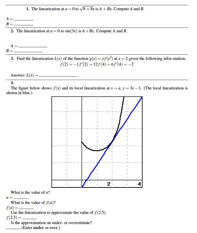
3. Find the linearization L(x) of the function g(x) =xf(x²) at x = 2 given the following infor-mation.
f (2) = -1f'(2) = 12f (4) = 6 f'(4) = -2
Answer: L(x) =.
4.
The figure below shows f(x) and its local linearization at x = a, y = 3x – 1. (The local linearization is
shown in blue.)
What is the value of a?
a =
What is the value of f(a)?
f(a) =-
Use the linearization to approximate the value of f(2.5).
f(2.5) =
Is the approximation an under- or overestimate?
(Enter under or over.)
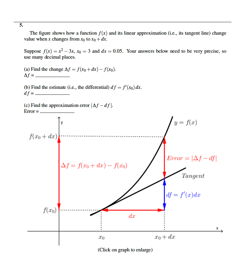
Transcribed Image Text:5.
The figure shows how a function f(x) and its linear approximation (i.e., its tangent line) change
value when x changes from xo to xo+dx.
Suppose f(x) = x² – 3x, xo = 3 and dx = 0.05. Your answers below need to be very precise, so
use many decimal places.
(a) Find the change Af = f(xo+dx) – f(xo).
Af =,
(b) Find the estimate (i.e., the differential) df = f'(xo) dx.
df = .
(c) Find the approximation error |Af –df\.
Error =.
y = f(x)
f(xo+ dx)
Error = |Af - df|
Af = f(x0+ dx) – f(xo)
Tangent
|df = f'(x)dx
f(xo)
dx
xo+ dx
(Click on graph to enlarge)
Expert Solution
This question has been solved!
Explore an expertly crafted, step-by-step solution for a thorough understanding of key concepts.


 Thomas' Calculus (14th Edition)CalculusISBN:9780134438986Author:Joel R. Hass, Christopher E. Heil, Maurice D. WeirPublisher:PEARSON
 Calculus: Early Transcendentals (3rd Edition)CalculusISBN:9780134763644Author:William L. Briggs, Lyle Cochran, Bernard Gillett, Eric SchulzPublisher:PEARSON
 Calculus: Early TranscendentalsCalculusISBN:9781319050740Author:Jon Rogawski, Colin Adams, Robert FranzosaPublisher:W. H. Freeman
 Calculus: Early Transcendental FunctionsCalculusISBN:9781337552516Author:Ron Larson, Bruce H. EdwardsPublisher:Cengage Learning