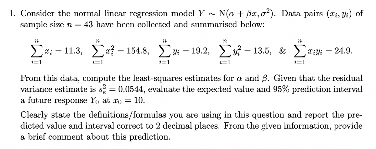
1. Consider the normal linear regression model Y~ N(a + Bx, o²). Data pairs (xi, yi) of sample size n= 43 have been collected and summarised below: n n n n n Σ |xi = 11.3, Σw = 154.8, Σy = 19.2, Σy =135, & Σαϊy = 24.9. i=1 i=1 i=1 i=1 i=1 From this data, compute the least-squares estimates for a and ß. Given that the residual variance estimate is s² = 0.0544, evaluate the expected value and 95% prediction interval a future response Yo at x = 10. Clearly state the definitions/formulas you are using in this question and report the pre- dicted value and interval correct to 2 decimal places. From the given information, provide a brief comment about this prediction.

The given quantities below were calculated from a sample data set. Στο 338 I Lu=308 Ση2 = 4678 2 y = 4236 Determine the least squares regression line. Round values to four decimal places, if necessary. Σry = 3595 n = 30 Determine the correlation coefficient. Round the solution to four decimal places, if necessary.

The temperatures (Observed and Expected) in centigrade for certain concrete mix sample have been presented as shown in the table below: Observed Expected Frequency Frequency 9 10 19 21 27 25 29 27 20 24 16 21 8 10 a- Use the data above to determine the Correlation Coefficient, between the Expected and the Observed frequencies b- Use the data above to determine the equation of the regression line between the expected and the observed frequencies. Note: Let the Observed values represent X and the Expected values represent Y.

After you estimate a simple linear regression you obtain the following sample regression function: Y₁ = 8.8 +0.7091 Xį With an r² of 0.784. The observed dependent variable used for the regression is: Y 9 675 40 40 40 6 5 5 5 5 1 1 Compute the sample variance of X? 8.45 10.79 9.17 7.19 Cannot be computed with the provided information.