MATLAB: An Introduction with Applications
6th Edition
ISBN: 9781119256830
Author: Amos Gilat
Publisher: John Wiley & Sons Inc
expand_more
expand_more
format_list_bulleted
Question
Please do the following questions in the image with R coding

Transcribed Image Text:6)
State the assumptions of the linear regression model.
7) L
Create the histogram of the residual and the residual plot. Comment assumption of the
linear regression model is satisfied or not.
8)
Use 1m () function in R and fit the regression model in 3) and use summary() function to
display output of 1m () function.
Again we use the model in 3). Use the output from 8) and do the test of hypothesis
Ho: B=0 vs H₁:8 +0.
Use a = 0.05. Then construct the 95% confidence interval of B.

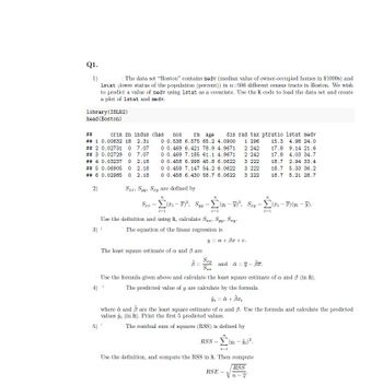
Transcribed Image Text:Q1.
1)
The data set "Boston" contains medv (median value of owner-occupied homes in $1000s) and
1stat (lower status of the population (percent)) in n-506 different census tracts in Boston. We wish
to predict a value of medv using 1stat as a covariate. Use the R code to load the data set and create
a plot of 1stat and medv.
11brary (ISLR2)
head (Boston)
##
crim zn indus chas
## 1 0.00632 18 2.31
## 2 0.02731 07.07
# # 3 0.02729 0 7.07
# # 4 0.03237 0 2.18
# # 5 0.06905 0 2.18
# # 6 0.02985 0 2.18
nox
rm age
0 0.538 6.575 65.2 4.0900
0 0.469 6.421 78.9 4.9671
0 0.469 7.185 61.1 4.9671
0 0.458 6.998 45.8 6.0622
0 0.458 7.147 54.2 6.0622
0 0.458 6.430 58.7 6.0622
2)
Szz, Syy, Sry are defined by
71
ST1 = (T-F)², Syy-i-)², Szy=(Ti-T) (Vi-T).
i=1
i=1
9.14 21.6
dis rad tax ptratio 1stat medv
1 296 15.3 4.98 24.0
2 242 17.8
2 242 17.8
3 222 18.7 2.94 33.4
3 222 18.7 5.33 36.2
3 222 18.7 5.21 28.7
4.03 34.7
=
The least square estimate of a and 3 are
i=1
Use the definition and using R, calculate Sr. Syy, Szy-
3) 1
The equation of the linear regression is
y = a + Br+e.
3= Szy and & = 7-8.
SII
Use the formula given above and calculate the least square estimate of a and 3 (in R).
The predicted value of y are calculate by the formula
91 = a + 3x₂
where à and 3 are the least square estimate of a and 3. Use the formula and calculate the predicted
values ; (in R). Print the first 5 predicted values.
The residual sum of squares (RSS) is defined by
n
Rss = Σ(m - 0;).
i=1
Use the definition, and compute the RSS in R. Then compute
RSS
RSE =
Vn-
Expert Solution
This question has been solved!
Explore an expertly crafted, step-by-step solution for a thorough understanding of key concepts.
Step by stepSolved in 5 steps with 5 images

Knowledge Booster
Similar questions
Recommended textbooks for you
 MATLAB: An Introduction with ApplicationsStatisticsISBN:9781119256830Author:Amos GilatPublisher:John Wiley & Sons Inc
 Probability and Statistics for Engineering and th...StatisticsISBN:9781305251809Author:Jay L. DevorePublisher:Cengage Learning
 Statistics for The Behavioral Sciences (MindTap C...StatisticsISBN:9781305504912Author:Frederick J Gravetter, Larry B. WallnauPublisher:Cengage Learning
 Elementary Statistics: Picturing the World (7th E...StatisticsISBN:9780134683416Author:Ron Larson, Betsy FarberPublisher:PEARSON
 The Basic Practice of StatisticsStatisticsISBN:9781319042578Author:David S. Moore, William I. Notz, Michael A. FlignerPublisher:W. H. Freeman
 Introduction to the Practice of StatisticsStatisticsISBN:9781319013387Author:David S. Moore, George P. McCabe, Bruce A. CraigPublisher:W. H. Freeman

MATLAB: An Introduction with Applications
Statistics
ISBN:9781119256830
Author:Amos Gilat
Publisher:John Wiley & Sons Inc

Probability and Statistics for Engineering and th...
Statistics
ISBN:9781305251809
Author:Jay L. Devore
Publisher:Cengage Learning

Statistics for The Behavioral Sciences (MindTap C...
Statistics
ISBN:9781305504912
Author:Frederick J Gravetter, Larry B. Wallnau
Publisher:Cengage Learning

Elementary Statistics: Picturing the World (7th E...
Statistics
ISBN:9780134683416
Author:Ron Larson, Betsy Farber
Publisher:PEARSON

The Basic Practice of Statistics
Statistics
ISBN:9781319042578
Author:David S. Moore, William I. Notz, Michael A. Fligner
Publisher:W. H. Freeman

Introduction to the Practice of Statistics
Statistics
ISBN:9781319013387
Author:David S. Moore, George P. McCabe, Bruce A. Craig
Publisher:W. H. Freeman