
MATLAB: An Introduction with Applications
6th Edition
ISBN: 9781119256830
Author: Amos Gilat
Publisher: John Wiley & Sons Inc
expand_more
expand_more
format_list_bulleted
Related questions
Question
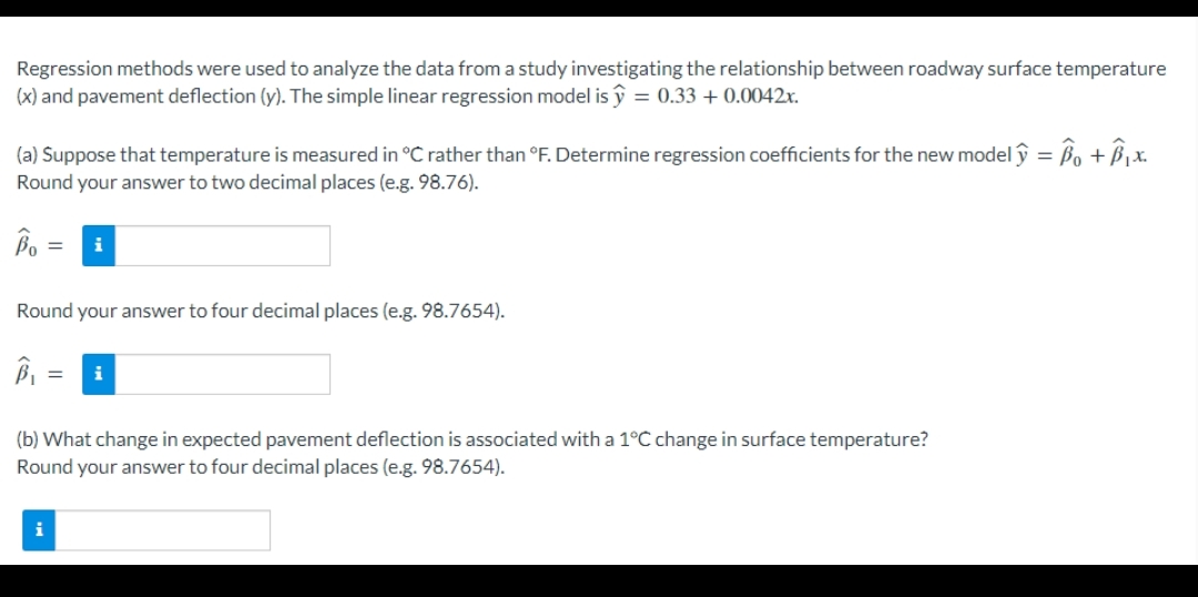

Transcribed Image Text:Regression methods were used to analyze the data from a study investigating the relationship between roadway surface temperature
(x) and pavement deflection (y). The simple linear regression model is ŷ = 0.33 + 0.0042x.
(a) Suppose that temperature is measured in °C rather than °F. Determine regression coefficients for the new model ŷ = ßo + B ¡x.
Round your answer to two decimal places (e.g. 98.76).
i
Round your answer to four decimal places (e.g. 98.7654).
(b) What change in expected pavement deflection is associated with a 1°C change in surface temperature?
Round your answer to four decimal places (e.g. 98.7654).
Expert Solution
This question has been solved!
Explore an expertly crafted, step-by-step solution for a thorough understanding of key concepts.

Step by stepSolved in 3 steps

Knowledge Booster

Similar questions
- 2. A high school track & field coach wanted to assess the relationship between an athletes height and how far they can jump in the long jump event (both in inches). They collect data on each athletes height and how far they can jump. Let the height in inches of the athlete be the explanatory variable (X) and the distance in inches of the jump be the response (Y). The scatterplot of the data based on 32 athletes is as follows: distance 88 86 84 82 80 78 00 O o 70 Scatter Plot 72 height 00 000 00 00 8 74 8 O ¥75 76 一念 78arrow_forwardmicroorganisms that break down these compounds. BOD is hard to measure accurately. Total organic carbon (TOC) is easy to measure, so it is common to measure TOC and use regression to predict BOD. A typical regression equation for water entering a municipal treatment plant is BOD= -55.42 + 1.507 TOC Both BOD and TOC are measured in milligrams per liter of water. (a) What does the slope of this line say about the relationship between BOD and TOC? O TOC rises (falls) by 1.507 mg/l for every 1 mg/l increase (decrease) in BOD O BOD rises (falls) by 1.507 mg/l for every 1 mg/l increase (decrease) in TOC O TOC rises (falls) by 1.507 mg/l for every 55.42 mg/l increase (decrease) in BOD O BOD rises (falls) by 55.42 mg/l for every 1 mg/l increase (decrease) in TOC (b) What is the predicted BOD when TOC = 0? Values of BOD less than 0 are impossible. Why do you think the prediction gives an impossible value? This arises from extrapolation; the data used to find this regression formula must not…arrow_forwardThe accompanying data are the number of wins and the earned run averages (mean number of earned runs allowed per nine innings pitched) for eight baseball pitchers in a recent season. Find the equation of the regression line. Then construct a scatter plot of the data and draw the regression line. Then use the regression equation to predict the value of y for each of the given x-values, if meaningful. If the x-value is not meaningful to predict the value of y, explain why not. (a) x = 5 wins (b) x = 10 wins (c) x = 19 wins (d) x = 15 wins E Click the icon to view the table of numbers of wins and earned run average. The equation of the regression line is y =x+ (Round to two decimal places as needed.) Construct a scatter plot of the data and draw the regression line. Choose the correct graph below. OA. OB. OC. OD. AERA 6- AERA AERA AERA 2- 2- 2- 0- 0- 12 18 24 12 18 24 12 18 24 12 18 24 Wins Wins Wins Wins (a) Predict the ERA for 5 wins, if it is meaningful. Select the correct choice below…arrow_forward
- Use the regression line to make the appropriate prediction. A random sample of records of electricity usage of homes in the month of July gives the amount of electricity used and size (in square feet) of 135 homes. A regression was done to predict the amount of eleçtricity used (in kilowatt-hours) (y) from size (x). The residuals plot indicated that a inear model is appropriate. The model is y = 0.2x+ 1271. How much electricity would you predict would be used in a house that is 2471 square feet? 494.2 kilowatt-hours O 6000.00 kilowatt-hours O 1765.2 kilowatt-hours O 776.8 kilowatt-hours 3742.2 kilowatt-hoursarrow_forwardThe accompanying data are the number of wins and the earned run averages (mean number of earned runs allowed per nine innings pitched) for eight baseball pitchers in a recent season. Find the equation of the regression line. Then construct a scatter plot of the data and draw the regression line. Then use the regression equation to predict the value of y for each of the given x-values, if meaningful. If the x-value is not meaningful to predict the value of y, explain why not. (a) x = 5 wins (b) x = 10 wins (c) x = 19 wins (d) x = 15 wins Click the icon to view the table of numbers of wins and earned run average. The equation of the regression line is y = x+. (Round to two decimal places as needed.)arrow_forwardMultiple regression analysis was used to study how an individual's income (Y in thousands of dollars) is influenced by age (X1 in years), level of education (X2 ranging from 1 to 5), and the person's gender (X3 where 0 =female and 1=male). The following is a partial result of computer output that was used on a sample of 20 individuals. Present the estimated regression equation and compute the coefficient of determination. Explain it. Use the t test to determine the significance of each independent variable. Let α = 0.05. (For each test, give the null and alternative hypotheses, test statistic, and conclusion.) Use the F test to determine whether or not the regression model is significant. Let α = 0.05. (For the test, give the null and alternative hypotheses, test statistic, and conclusion.) Does the estimated regression equation provide a good fit for the observed data? Explain it. Suppose a new person with X1=40, X2=4, X3=0. Use the estimated regression equation in part (a)…arrow_forward
- The accompanying data are the number of wins and the earned run averages (mean number of earned runs allowed per nine innings pitched) for eight baseball pitchers in a recent season. Find the equation of the regression line. Then construct a scatter plot of the data and draw the regression line. Then use the regression equation to predict the value of y for each of the given x-values, if meaningful. If the x-value is not meaningful to predict the value of y, explain why not. (a) x = 5 wins (c) x = 19 wins (d) x = 15 wins (b)x= 10 wins Click the icon to view the table of numbers of wins and earned run average. .. The equation of the regression line is y=x+ X+ (Round to two decimal places as needed.) Construct a scatter plot of the data and draw the regression line. Choose the correct graph below. OA. B. O C. O D. AERA AERA 6+ Q AERA 6+ 4- 4- 2- 2- 0- 6 12 18 24 0 12 18 24 6 12 18 24 Wins 12 18 24 Wins Wins Wins (a) Predict the ERA for 5 wins, if it is meaningful. Select the correct…arrow_forwardA real estate company wants to study the relationship between house sales prices and some important predictors of sales prices. Based on data from recently sold homes in the space, the following variables are used in a multiple regression model. y = sales price (in thousands of dollars) x₁ = total floor area (in square feet) x₂ = number of bedrooms x3 distance to nearest high school (in miles) = The estimated model is as follows. =76+0.098x₁ +16x₂ - 8x3 Answer the questions below for the interpretation of the coefficient of X₂ in this model. (a) Holding the other variables fixed, what is the average change in sales price for each additional bedroom in a house? dollars (b) Is this change an increase or a decrease? O increase O decrease Xarrow_forwardThe age and height (in cm) of 400 adult women from Bolivia were measured. A researcher wants to know if age has any effect on height. A linear regression is carried out in Minitab and the following output obtained. Coefficients Term Constant Age (a) Write down the regression model. (b) Interpret the regression coefficient for the fitted model. (c) Use the output from Minitab to explain if the age of a participant affects their height. Percent (d) The normal probability plot of the residuals from this regression model is given below. Do the assumptions of the regression model seem reasonable? Justify your answer. 99.9 8 28 22299229 88 Coef SE Coef 152.94 7.69 0.022 0.231 01 -100 T-Value P-Value VIF 19.90 0.000 0.10 0.924 1.00 -50 Normal Probability Plot (response is Height) 0 Residual 50 ***** 100 150arrow_forward
- A regression analysis was performed to determine if there is a relationship between hours of TV watched per day (xx) and number of sit ups a person can do (yy). The results of the regression were: y=ax+b a=-1.152 b=30.418 r2=0.703921 r=-0.839 1. Use this to predict the number of sit ups a person who watches 2.5 hours of TV can do, and please round your answer to a whole numberarrow_forwardThe accompanying data are the number of wins and the earned run averages (mean number of earned runs allowed per nine innings pitched) for eight baseball pitchers in a recent season. Find the equation of the regression line. Then construct a scatter plot of the data and draw the regression line. Then use the regression equation to predict the value of y for each of the given x-values, if meaningful. If the x-value is not meaningful to predict the value of y, explain why not. (a) x= 5 wins E Click the icon to view the table of numbers of wins and earned run average. (b) x = 10 wins (c) x = 19 wins (d) x= 15 wins ..... The equation of the regression line is y = x+O (Round to two decimal places as needed.) Wins and ERA Earned run Wins, x average, y 20 2.71 18 3.19 17 2.69 16 3.68 14 3.94 12 4.25 11 3.86 9 5.18 Print Donearrow_forwardResearchers are interested in predicting the height of a child based on the heights of their mother and father. Data were collected, which included height of the child ( height), height of the mother ( mothersheight ), and height of the father (fathersheight ). The initial analysis used the heights of the parents to predict the height of the child (all units are inches). The results of the analysis, a multiple regression, are presented below. . regress height mothersheight fathersheight Source Model Residual Total height mothersheight fathersheight _cons SS 208.008457 314.295372 522.303829 df 2 104.004228 8.49446952 37 MS 39 13.3924059 Coef. Std. Err. .6579529 .1474763 .2003584 .1382237 9.804327 12.39987 t P>|t| 4.46 0.000 C 0.156 0.79 0.434 Number of obs = F( 2, 37) = Prob > F R-squared Adj R-squared = Root MSE = = .3591375 -.0797093 -15.32021 = 40 12.24 0.0001 0.3983 0.3657 2.9145 [95% Conf. Interval] .9567683 .4804261 34.92886 What are the null and alternative hypotheses…arrow_forward
arrow_back_ios
SEE MORE QUESTIONS
arrow_forward_ios
Recommended textbooks for you
- MATLAB: An Introduction with ApplicationsStatisticsISBN:9781119256830Author:Amos GilatPublisher:John Wiley & Sons Inc
 Probability and Statistics for Engineering and th...StatisticsISBN:9781305251809Author:Jay L. DevorePublisher:Cengage Learning
 Statistics for The Behavioral Sciences (MindTap C...StatisticsISBN:9781305504912Author:Frederick J Gravetter, Larry B. WallnauPublisher:Cengage Learning
  Elementary Statistics: Picturing the World (7th E...StatisticsISBN:9780134683416Author:Ron Larson, Betsy FarberPublisher:PEARSON
 The Basic Practice of StatisticsStatisticsISBN:9781319042578Author:David S. Moore, William I. Notz, Michael A. FlignerPublisher:W. H. Freeman
 Introduction to the Practice of StatisticsStatisticsISBN:9781319013387Author:David S. Moore, George P. McCabe, Bruce A. CraigPublisher:W. H. Freeman
MATLAB: An Introduction with Applications
Statistics
ISBN:9781119256830
Author:Amos Gilat
Publisher:John Wiley & Sons Inc
Probability and Statistics for Engineering and th...
Statistics
ISBN:9781305251809
Author:Jay L. Devore
Publisher:Cengage Learning
Statistics for The Behavioral Sciences (MindTap C...
Statistics
ISBN:9781305504912
Author:Frederick J Gravetter, Larry B. Wallnau
Publisher:Cengage Learning
Elementary Statistics: Picturing the World (7th E...
Statistics
ISBN:9780134683416
Author:Ron Larson, Betsy Farber
Publisher:PEARSON
The Basic Practice of Statistics
Statistics
ISBN:9781319042578
Author:David S. Moore, William I. Notz, Michael A. Fligner
Publisher:W. H. Freeman
Introduction to the Practice of Statistics
Statistics
ISBN:9781319013387
Author:David S. Moore, George P. McCabe, Bruce A. Craig
Publisher:W. H. Freeman