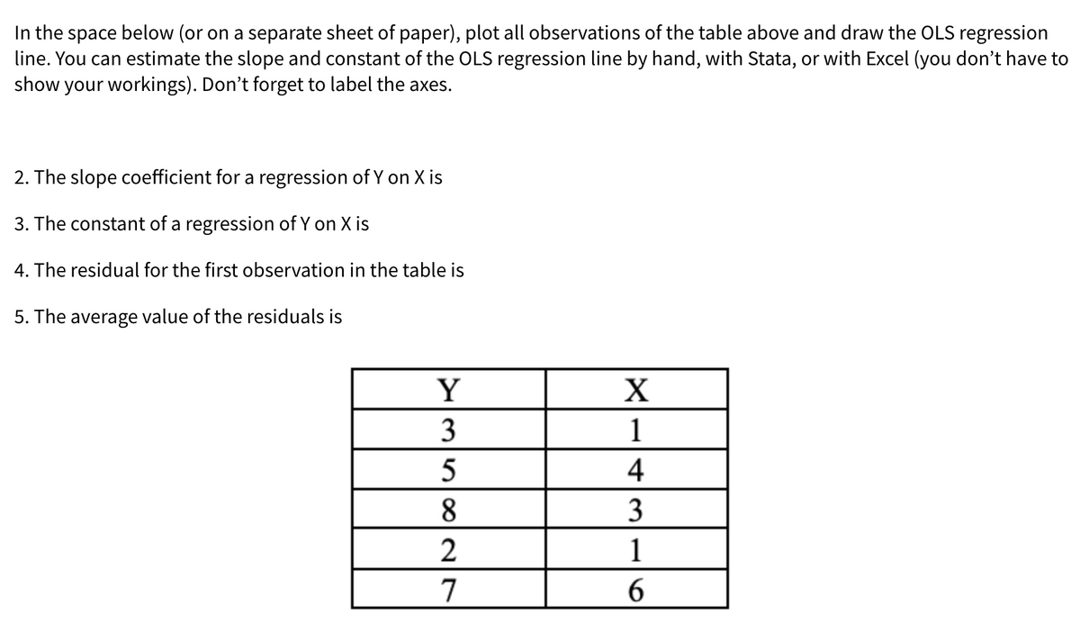
In the space below (or on a separate sheet of paper), plot all observations of the table above and draw the OLS regression line. You can estimate the slope and constant of the OLS regression line by hand, with Stata, or with Excel (you don't have to show your workings). Don't forget to label the axes. 2. The slope coefficient for a regression of Y on X is 3. The constant of a regression of Y on X is 4. The residual for the first observation in the table is 5. The average value of the residuals is Y X 3 1 5 4 3 2 1 7 6.

Please solve what’s not filled in.

The data show the chest size and weight of several bears. Find the regression equation, letting chest size be the independent (x) variable. Then find the best predicted weight of a bear with a chest size of 63 inches. Is the result close to the actual weight of 522 pounds? Use a significance level of 0.05. Chest size (inches) 58 50 65 59 59 48 D 414 312 499 450 456 260 Weight (pounds) Click the icon to view the critical values of the Pearson correlation coefficient r. What is the regression equation? y=+x (Round to one decimal place as needed.) What is the best predicted weight of a bear with a chest size of 63 inches? The best predicted weight for a bear with a chest size of 63 inches is pounds. (Round to one decimal place as needed.) Is the result close to the actual weight of 522 pounds? O A. This result is not very close to the actual weight of the bear. O B. This result is exactly the same as the actual weight of the bear. O C. This result is close to the actual weight of the…

Which of the following is true of a linear regression line? a.  Located as close as possible to all the points of a scatter chart. B.  Is defined by an equation having 2 parameters: the slope and the intercept c.  Provides an approximate relationship between the values of two parameters d.  All of the above

Part a: Make a scatter plot and determine which type of model best fits the data.Part b: Find the regression equation.Part c: Use the equation from Part b to determine y when x = 1.5.

Lesson Plan Revi..pdf MacBook Pro 4. A farmer has a flock of turkeys with weights that are normally distributed with a mean of 15.3 pounds and a standard deviation of 2.3 pounds. If one turkey is selected at random, wha weight is less than 17.0 pounds? is the probability that its

A newspaper article reported that 320 people in one state were surveyed and 80% were opposed to a recent court decision. The same article reported that a similar survey of 510 people in another state indicated opposition by only 30%. Construct a 99% confidence interval of the difference in population proportions based on the data. The 99% confidence interval of the difference in population proportions is ( (Round to four decimal places as needed.)