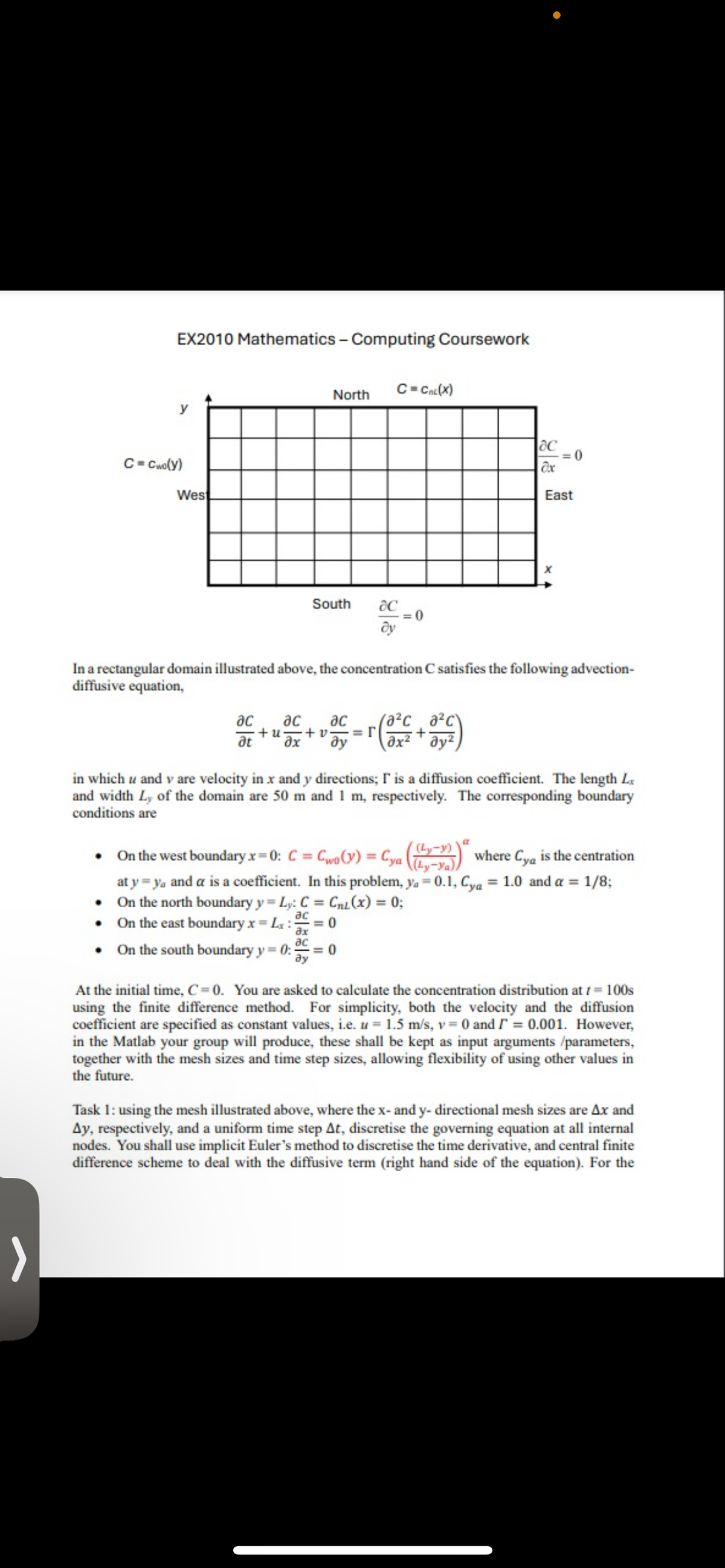
EX2010 Mathematics - Computing Coursework C-Cwo(y) West North C=Cnc (X) South дс = 0 By Oc =0 ax East x In a rectangular domain illustrated above, the concentration C satisfies the following advection- diffusive equation, ac ac (a²c a²c\ ас at ax +u+v. =Г ду + in which u and v are velocity in x and y directions; I' is a diffusion coefficient. The length L and width Ly of the domain are 50 m and 1 m, respectively. The corresponding boundary conditions are a On the west boundary x=0: C = Cwo(y) = Cya (y-1)) where Cya is the centration at y ya and a is a coefficient. In this problem, ya=0.1, Cya = 1.0 and α = 1/8; ⚫ On the north boundary y = Ly: C ⚫ On the east boundary x = Lx: = 0 = CnL(x) = 0; ac ax ⚫ On the south boundary y = 0:3 дс = 0 ay At the initial time, C=0. You are asked to calculate the concentration distribution at /= 100s using the finite difference method. For simplicity, both the velocity and the diffusion coefficient are specified as constant values, i.e. u = 1.5 m/s, v = 0 and = 0.001. However, in the Matlab your group will produce, these shall be kept as input arguments /parameters, together with the mesh sizes and time step sizes, allowing flexibility of using other values in the future. Task 1: using the mesh illustrated above, where the x- and y- directional mesh sizes are Ax and Ay, respectively, and a uniform time step At, discretise the governing equation at all internal nodes. You shall use implicit Euler's method to discretise the time derivative, and central finite difference scheme to deal with the diffusive term (right hand side of the equation). For the

EX2010 Mathematics - Computing Coursework C-Cwo(y) West North C=Cnc (X) South дс = 0 By Oc =0 ax East x In a rectangular domain illustrated above, the concentration C satisfies the following advection- diffusive equation, ac ac (a²c a²c\ ас at ax +u+v. =Г ду + in which u and v are velocity in x and y directions; I' is a diffusion coefficient. The length L and width Ly of the domain are 50 m and 1 m, respectively. The corresponding boundary conditions are a On the west boundary x=0: C = Cwo(y) = Cya (y-1)) where Cya is the centration at y ya and a is a coefficient. In this problem, ya=0.1, Cya = 1.0 and α = 1/8; ⚫ On the north boundary y = Ly: C ⚫ On the east boundary x = Lx: = 0 = CnL(x) = 0; ac ax ⚫ On the south boundary y = 0:3 дс = 0 ay At the initial time, C=0. You are asked to calculate the concentration distribution at /= 100s using the finite difference method. For simplicity, both the velocity and the diffusion coefficient are specified as constant values, i.e. u = 1.5 m/s, v = 0 and = 0.001. However, in the Matlab your group will produce, these shall be kept as input arguments /parameters, together with the mesh sizes and time step sizes, allowing flexibility of using other values in the future. Task 1: using the mesh illustrated above, where the x- and y- directional mesh sizes are Ax and Ay, respectively, and a uniform time step At, discretise the governing equation at all internal nodes. You shall use implicit Euler's method to discretise the time derivative, and central finite difference scheme to deal with the diffusive term (right hand side of the equation). For the