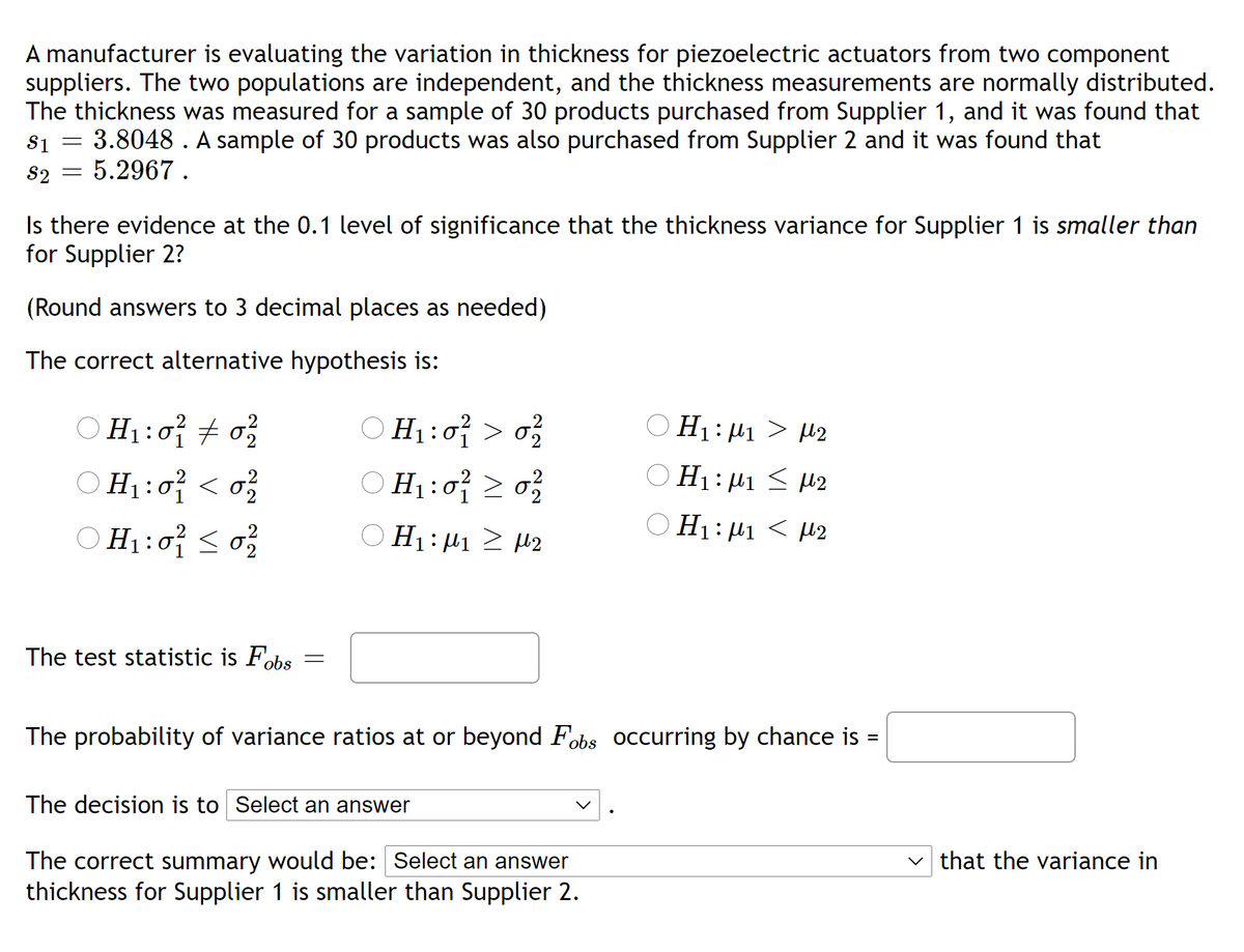
A manufacturer is evaluating the variation in thickness for piezoelectric actuators from two component suppliers. The two populations are independent, and the thickness measurements are normally distributed. The thickness was measured for a sample of 30 products purchased from Supplier 1, and it was found that s1 = 3.8048 . A sample of 30 products was also purchased from Supplier 2 and it was found that 82 = 5.2967. Is there evidence at the 0.1 level of significance that the thickness variance for Supplier 1 is smaller than for Supplier 2? (Round answers to 3 decimal places as needed) The correct alternative hypothesis is: O H1:0 + o O H1:0} < o? O H1:0} < o H1:0 > o? H1: 41 > H2 H1: µ1 < H2 H1: µ1 2 H2 H1: µ1 < µ2 The test statistic is Fobs The probability of variance ratios at or beyond Fobs occurring by chance is = The decision is to Select an answer v that the variance in The correct summary would be: Select an answer thickness for Supplier 1 is smaller than Supplier 2.

To compare the dry braking distances from 30 to 0 miles per hour for two makes of​ automobiles, a safety engineer conducts braking tests for 35 models of Make A and 35 models of Make B. The mean braking distance for Make A is 43 feet. Assume the population standard deviation is 4.6 feet. The mean braking distance for Make B is 46 feet. Assume the population standard deviation is 4.5 feet. At α=0.10​, can the engineer support the claim that the mean braking distances are different for the two makes of​ automobiles? Assume the samples are random and​ independent, and the populations are normally distributed.   The critical​ value(s) is/are   Find the standardized test statistic z for μ1−μ2.

Given the Z scores of: -1.5, 0.52, -1.0, 1.7 and 3.0:  1. Calculate the raw skewness and kurtosis scores for these data. 2. Calculate the standard error scores for skewness and kurtosis for these data. 3. Calculate the Z scores for skewness and kurtosis for these data.

In a certain article, laser therapy was discussed as a useful alternative to drugs in pain management of chronically ill patients. To measure pain threshold, a machine was used that delivered low-voltage direct current to different parts of the body (wrist, neck, and back). The machine measured current in milliamperes (mA). The pretreatment experimental group in the study had an average threshold of pain (pain was first detectable) at u = 3.30 mA with standard deviation o = 1.23 mA. Assume that the distribution of threshold pain, measured in milliamperes, is symmetric and more or less mound-shaped. (Round your answers to two decimal places.) (a) Use the empirical rule to estimate a range of milliamperes centered about the mean in which about 68% of the experimental group will have a threshold of pain from mA to (b) Use the empirical rule to estimate a range of milliamperes centered about the mean in which about 95% of the experimental group will have a threshold of pain from mA to mA

A random sample of n1 = 20 winter days in Denver gave a sample mean pollution index x1 = 43. Previous studies show that σ1 = 11. For Englewood (a suburb of Denver), a random sample of n2 = 10 winter days gave a sample mean pollution index of x2 = 31. Previous studies show that σ2 = 18. Assume the pollution index is normally distributed in both Englewood and Denver. Do these data indicate that the mean population pollution index of Englewood is different (either way) from that of Denver in the winter? Use a 1% level of significance. (a) What is the level of significance?   State the null and alternate hypotheses. H0: μ1 < μ2; H1: μ1 = μ2H0: μ1 = μ2; H1: μ1 > μ2    H0: μ1 = μ2; H1: μ1 ≠ μ2H0: μ1 = μ2; H1: μ1 < μ2 (b) What sampling distribution will you use? What assumptions are you making? The standard normal. We assume that both population distributions are approximately normal with unknown standard deviations.The Student's t. We assume that both population…

An engineer wants to know if producing metal bars using a new experimental treatment rather than the conventional treatment makes a difference in the tensile strength of the bars​ (the ability to resist tearing when pulled​ lengthwise). At α=0.10​, answer parts​ (a) through​ (e). Assume the population variances are equal and the samples are random. If​ convenient, use technology to solve the problem.   Treatment Tensile strengths (newtons per square millimeter) Experimental 449 354 450 360 433 388 400                       Conventional 370 376 374 424 378 450 438 404 352 376   ​(a) Identify the claim and state H0 and Ha.   The claim is​ "The new treatment ▼   makes a difference does not make a difference in the tensile strength of the​ bars." What are H0 and Ha​?   The null​ hypothesis, H0​, is ▼   mu 1 equals mu 2μ1=μ2 mu 1 less than or equals mu 2μ1≤μ2 mu 1 greater than or equals mu 2μ1≥μ2 . The alternative​ hypothesis, Ha​,…

The length (in mm) of a spring subjected to a force FNewtons is of the form L = a + BF+ ɛ, where ɛ is assumed normally distributed with mean 0, variance o2. Given the sample statisticsn=D13, E F;= 138, E L; = 577, SEL = -43, SEF= 1735, estimate the expected length of the spring when a force of 11.2 Newtons is applied. (Give your answer correct to 2 decimal places.) Answer: Ti Check 江一 prime viden Type here to search 19 hp ins prt fu f12 f8 f9 f10 f7 f5 f6 『米 " JOI JDI & 6 7 8 5 96 %24 3

A random sample of size 36 from a population with known variance, o = 9, yields a sample mean of x = 17. Find ß, for testing the hypothesis H,: u = 15 versus H1 : =16. Assume a 0.05. %3D %3D

Consider the demand for Fresh Detergent in a future sales period when Enterprise Industries' price for Fresh will be x1 = 3.70, the average price of competitors' similar detergents will be x2 = 3.90, and Enterprise Industries' advertising expenditure for Fresh will be x3 = 6.50. A 95 percent prediction interval for this demand is given on the following JMP output: %3D Predicted Lower 95% Upper 95% Mean Demand Upper 95% Indiv Demand StdErr Lower 95% Demand Mean Demand Indiv Demand Indiv Demand 31 8.4106503477 8.3143172822 8.5069834132 0.2393033103 7.9187553487 8.9025453468 E Click here for the Excel Data File; (a) Find and report the 95 percent prediction interval on the output. If Enterprise Industries plans to have in inventory the number of bottles implied by the upper limit of this interval, it can be very confident that it will have enough bottles to meet demand for Fresh in the future sales period. How many bottles is this? If we multiply the number of bottles implied by the lower…

An engineer measures the peak current (in microamps) when a solution containing an amount of nickel (in parts per 10°) is added to a buffer. The experiment was repeated for eleven different values of nickel solutions. A scatterplot showing the data is given below: Peak Current in Eleven Buffers with Added Nickel Solutio 60 120 140 100 Amount of nickel (pp million) Suppose a regression line was added to the plot above. If an additional measurement had been taken with the nickel of 62 parts per 10 and a peak current of 0.38 microamps, adding this observation would: O A. increase the intercept, decrease the slope. OB. increase the intercept, increase the slope. C. decrease the intercept, increase the slope. OD. decrease the intercept, decrease the slope. E. not affect the regression line.