%%% plotting the solution y for each gamma figure; = gamma 0.2; [t,y] ode45(@(t, y) mass_spring_ext(t,y,gamma), [0 100], [1; 0]); plot(t,y(:,1), '+'); hold on; 6 7 8 9 10 11 12 13 14 [t,y] => 15 16 gamma 0.42; ode45(@(t,y) mass_spring_ext(t,y,gamma), [0 100], [1; 0]); plot(t,y(:,1),'-'); hold on; gamma = 0.6; ode45 (@(t,y) mass_spring_ext(t,y, t,y,gamma), [0 100],[1; 0]); plot(t,y(:,1),'-o'); hold on; ode45 (@(t, y) mass_spring_ext(t,y,gamma), [0 100], [1; 0]); 17 18 [t,y] = 19 20 21 gamma 0.8; 22 [t,y] 23 24 25 26 27 28 29 plot(t,y(:,1), ); hold off; xlabel( Time t'); ylabel('Solution y'); legend (gamma-0.2', 'gamma-0.42', 'gamma-0.6', 'gamma-0.8'); 30 Ε 31 32 33 34 35 36 37 38 %%%% %%% plotting the amplitude of the steady-state solution (A(gamma)-FO*M(gamma)) vs gamma figure; = = m= 1; k 1/5; b 1/5; F0 = 1; gama = 0.2:0.01:0.8; M_gama FO./sqrt((k-m*gama. ^2).^2+b^2*gama. ^2); plot (gama, M_gama); xlabel('gamma'); ylabel('A(gamma)'); 1. A mass-spring motion is governed by the ordinary differential equation d²x dx m. +b dt² dt +k(t)x = F(t), where m is the mass, b is the damping constant, k is the spring constant, and F(t) is the external force. We consider the initial conditions x(0): = 1 and x'(0) = 0. Assume the following numerical values for this part of the project: m = 1, k = 1/4, b=1/5, and F(t) = sin yt. (a) Read section 4.10. Explain what is the resonance frequency, and then compute the resonance frequency for this mass-spring system. (b) The ODE45-solver can be used to obtain the solution curves in MATLAB. Use the script Project2_Q1.m to plot the solutions and estimate the amplitude A of the steady response for Y === 0.25, 0.45, 0.65, and 0.85. (c) The script also provide you with the graph of A versus y. For what frequency y is the amplitude the greatest? Is it equal to that you obtained in (a)?
%%% plotting the solution y for each gamma figure; = gamma 0.2; [t,y] ode45(@(t, y) mass_spring_ext(t,y,gamma), [0 100], [1; 0]); plot(t,y(:,1), '+'); hold on; 6 7 8 9 10 11 12 13 14 [t,y] => 15 16 gamma 0.42; ode45(@(t,y) mass_spring_ext(t,y,gamma), [0 100], [1; 0]); plot(t,y(:,1),'-'); hold on; gamma = 0.6; ode45 (@(t,y) mass_spring_ext(t,y, t,y,gamma), [0 100],[1; 0]); plot(t,y(:,1),'-o'); hold on; ode45 (@(t, y) mass_spring_ext(t,y,gamma), [0 100], [1; 0]); 17 18 [t,y] = 19 20 21 gamma 0.8; 22 [t,y] 23 24 25 26 27 28 29 plot(t,y(:,1), ); hold off; xlabel( Time t'); ylabel('Solution y'); legend (gamma-0.2', 'gamma-0.42', 'gamma-0.6', 'gamma-0.8'); 30 Ε 31 32 33 34 35 36 37 38 %%%% %%% plotting the amplitude of the steady-state solution (A(gamma)-FO*M(gamma)) vs gamma figure; = = m= 1; k 1/5; b 1/5; F0 = 1; gama = 0.2:0.01:0.8; M_gama FO./sqrt((k-m*gama. ^2).^2+b^2*gama. ^2); plot (gama, M_gama); xlabel('gamma'); ylabel('A(gamma)'); 1. A mass-spring motion is governed by the ordinary differential equation d²x dx m. +b dt² dt +k(t)x = F(t), where m is the mass, b is the damping constant, k is the spring constant, and F(t) is the external force. We consider the initial conditions x(0): = 1 and x'(0) = 0. Assume the following numerical values for this part of the project: m = 1, k = 1/4, b=1/5, and F(t) = sin yt. (a) Read section 4.10. Explain what is the resonance frequency, and then compute the resonance frequency for this mass-spring system. (b) The ODE45-solver can be used to obtain the solution curves in MATLAB. Use the script Project2_Q1.m to plot the solutions and estimate the amplitude A of the steady response for Y === 0.25, 0.45, 0.65, and 0.85. (c) The script also provide you with the graph of A versus y. For what frequency y is the amplitude the greatest? Is it equal to that you obtained in (a)?

C++ for Engineers and Scientists
4th Edition
ISBN:9781133187844
Author:Bronson, Gary J.
Publisher:Bronson, Gary J.
Chapter7: Arrays
Section7.5: Case Studies
Problem 15E

Related questions
Question
Please solve using the script attached in the picture.
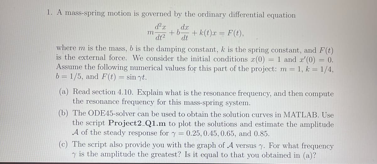
![%%% plotting the solution y for each gamma
figure;
=
gamma 0.2;
[t,y] ode45(@(t, y) mass_spring_ext(t,y,gamma), [0 100], [1; 0]);
plot(t,y(:,1), '+'); hold on;
6
7
8
9
10
11
12
13
14
[t,y]
=>
15
16
gamma
0.42;
ode45(@(t,y) mass_spring_ext(t,y,gamma), [0 100], [1; 0]);
plot(t,y(:,1),'-'); hold on;
gamma = 0.6;
ode45 (@(t,y) mass_spring_ext(t,y,
t,y,gamma), [0 100],[1; 0]);
plot(t,y(:,1),'-o'); hold on;
ode45 (@(t, y) mass_spring_ext(t,y,gamma), [0 100], [1; 0]);
17
18
[t,y]
=
19
20
21
gamma
0.8;
22
[t,y]
23
24
25
26
27
28
29
plot(t,y(:,1), ); hold off;
xlabel( Time t');
ylabel('Solution y');
legend (gamma-0.2', 'gamma-0.42', 'gamma-0.6', 'gamma-0.8');
30 Ε
31
32
33
34
35
36
37
38
%%%%
%%% plotting the amplitude of the steady-state solution (A(gamma)-FO*M(gamma)) vs gamma
figure;
=
=
m= 1; k 1/5; b 1/5; F0 = 1;
gama = 0.2:0.01:0.8;
M_gama FO./sqrt((k-m*gama. ^2).^2+b^2*gama. ^2);
plot (gama, M_gama);
xlabel('gamma');
ylabel('A(gamma)');](/v2/_next/image?url=https%3A%2F%2Fcontent.bartleby.com%2Fqna-images%2Fquestion%2F5e996ea7-cb36-40c1-90ef-5b50ce800a3d%2Ff72ae16a-83c2-40cf-b761-bd8bf5ad138a%2Fcc9h7eg_processed.jpeg&w=3840&q=75)
Transcribed Image Text:%%% plotting the solution y for each gamma
figure;
=
gamma 0.2;
[t,y] ode45(@(t, y) mass_spring_ext(t,y,gamma), [0 100], [1; 0]);
plot(t,y(:,1), '+'); hold on;
6
7
8
9
10
11
12
13
14
[t,y]
=>
15
16
gamma
0.42;
ode45(@(t,y) mass_spring_ext(t,y,gamma), [0 100], [1; 0]);
plot(t,y(:,1),'-'); hold on;
gamma = 0.6;
ode45 (@(t,y) mass_spring_ext(t,y,
t,y,gamma), [0 100],[1; 0]);
plot(t,y(:,1),'-o'); hold on;
ode45 (@(t, y) mass_spring_ext(t,y,gamma), [0 100], [1; 0]);
17
18
[t,y]
=
19
20
21
gamma
0.8;
22
[t,y]
23
24
25
26
27
28
29
plot(t,y(:,1), ); hold off;
xlabel( Time t');
ylabel('Solution y');
legend (gamma-0.2', 'gamma-0.42', 'gamma-0.6', 'gamma-0.8');
30 Ε
31
32
33
34
35
36
37
38
%%%%
%%% plotting the amplitude of the steady-state solution (A(gamma)-FO*M(gamma)) vs gamma
figure;
=
=
m= 1; k 1/5; b 1/5; F0 = 1;
gama = 0.2:0.01:0.8;
M_gama FO./sqrt((k-m*gama. ^2).^2+b^2*gama. ^2);
plot (gama, M_gama);
xlabel('gamma');
ylabel('A(gamma)');
Transcribed Image Text:1. A mass-spring motion is governed by the ordinary differential equation
d²x dx
m. +b
dt² dt
+k(t)x = F(t),
where m is the mass, b is the damping constant, k is the spring constant, and F(t)
is the external force. We consider the initial conditions x(0): = 1 and x'(0) = 0.
Assume the following numerical values for this part of the project: m = 1, k = 1/4,
b=1/5, and F(t) = sin yt.
(a) Read section 4.10. Explain what is the resonance frequency, and then compute
the resonance frequency for this mass-spring system.
(b) The ODE45-solver can be used to obtain the solution curves in MATLAB. Use
the script Project2_Q1.m to plot the solutions and estimate the amplitude
A of the steady response for Y === 0.25, 0.45, 0.65, and 0.85.
(c) The script also provide you with the graph of A versus y. For what frequency
y is the amplitude the greatest? Is it equal to that you obtained in (a)?
Expert Solution
This question has been solved!
Explore an expertly crafted, step-by-step solution for a thorough understanding of key concepts.

This is a popular solution!

Trending now
This is a popular solution!

Step by step
Solved in 1 steps with 2 images

Recommended textbooks for you
C++ for Engineers and Scientists
Computer Science
ISBN:
9781133187844
Author:
Bronson, Gary J.
Publisher:
Course Technology Ptr

Operations Research : Applications and Algorithms
Computer Science
ISBN:
9780534380588
Author:
Wayne L. Winston
Publisher:
Brooks Cole
C++ for Engineers and Scientists
Computer Science
ISBN:
9781133187844
Author:
Bronson, Gary J.
Publisher:
Course Technology Ptr
Operations Research : Applications and Algorithms
Computer Science
ISBN:
9780534380588
Author:
Wayne L. Winston
Publisher:
Brooks Cole